For the 36th Time… the Latest from Our R&D Pipeline
Today we celebrate the arrival of the 36th (x.x) version of the Wolfram Language and Mathematica: Version 14.1. We’ve been doing this since 1986: continually inventing new ideas and implementing them in our larger and larger tower of technology. And it’s always very satisfying to be able to deliver our latest achievements to the world.
We released Version 14.0 just half a year ago. And—following our modern version scheduling—we’re now releasing Version 14.1. For most technology companies a .1 release would contain only minor tweaks. But for us it’s a snapshot of what our whole R&D pipeline has delivered—and it’s full of significant new features and new enhancements.
If you’ve been following our livestreams, you may have already seen many of these features and enhancements being discussed as part of our open software design process. And we’re grateful as always to members of the Wolfram Language community who’ve made suggestions—and requests. And in fact Version 14.1 contains a particularly large number of long-requested features, some of which involved development that has taken many years and required many intermediate achievements.
There’s lots of both extension and polishing in Version 14.1. There are a total of 89 entirely new functions—more than in any other version for the past couple of years. And there are also 137 existing functions that have been substantially updated. Along with more than 1300 distinct bug fixes and specific improvements.
Some of what’s new in Version 14.1 relates to AI and LLMs. And, yes, we’re riding the leading edge of these kinds of capabilities. But the vast majority of what’s new has to do with our continued mission to bring computational language and computational knowledge to everything. And today that mission is even more important than ever, supporting not only human users, but also rapidly proliferating AI “users”—who are beginning to be able to routinely make even broader and deeper use of our technology than humans.
Each new version of Wolfram Language represents a large amount of R&D by our team, and the encapsulation of a surprisingly large number of ideas about what should be implemented, and how it should be implemented. So, today, here it is: the latest stage in our four-decade journey to bring the superpower of the computational paradigm to everything.
There’s Now a Unified Wolfram App
In the beginning we just had “Mathematica”—that we described as “A System for Doing Mathematics by Computer”. But the core of “Mathematica”—based on the very general concept of transformations for symbolic expressions—was always much broader than “mathematics”. And it didn’t take long before “mathematics” was an increasingly small part of the system we had built. We agonized for years about how to rebrand things to better reflect what the system had become. And eventually, just over a decade ago, we did the obvious thing, and named what we had “the Wolfram Language”.
But when it came to actual software products and executables, so many people were familiar with having a “Mathematica” icon on their desktop that we didn’t want to change that. Later we introduced Wolfram|One as a general product supporting Wolfram Language across desktop and cloud—with Wolfram Desktop being its desktop component. But, yes, it’s all been a bit confusing. Ultimately there’s just one “bag of bits” that implements the whole system we’ve built, even though there are different usage patterns, and differently named products that the system supports. Up to now, each of these different products has been a different executable, that’s separately downloaded.
But starting with Version 14.1 we’re unifying all these things—so that now there’s just a single unified Wolfram app, that can be configured and activated in different ways corresponding to different products.
So now you just go to wolfram.com/download-center and download the Wolfram app:
![]()
After you’ve installed the app, you activate it as whatever product(s) you’ve got: Wolfram|One, Mathematica, Wolfram|Alpha Notebook Edition, etc. Why have separate products? Each one has a somewhat different usage pattern, and provides a somewhat different interface optimized for that usage pattern. But now the actual downloading of bits has been unified; you just have to download the unified Wolfram app and you’ll get what you need.
Vector Databases and Semantic Search
Let’s say you’ve got a million documents (or webpages, or images, or whatever) and you want to find the ones that are “closest” to something. Version 14.1 now has a function—SemanticSearch—for doing this. How does SemanticSearch work? Basically it uses machine learning methods to find “vectors” (i.e. lists) of numbers that somehow represent the “meaning” of each of your documents. Then when you want to know which documents are “closest” to something, SemanticSearch computes the vector for the something, and then sees which of the document vectors are closest to this vector.
In principle one could use Nearest to find closest vectors. And indeed this works just fine for small examples where one can readily store all the vectors in memory. But SemanticSearch uses a full industrial-strength approach based on the new vector database capabilities of Version 14.1—which can work with huge collections of vectors stored in external files.
There are lots of ways to use both SemanticSearch and vector databases. You can use them to find documents, snippets within documents, images, sounds or anything else whose “meaning” can somehow be captured by a vector of numbers. Sometimes the point is to retrieve content directly for human consumption. But a particularly strong modern use case is to set up “retrieval-augmented generation” (RAG) for LLMs—in which relevant content found with a vector database is used to provide a “dynamic prompt” for the LLM. And indeed in Version 14.1—as we’ll discuss later—we now have LLMPromptGenerator to implement exactly this pipeline.
But let’s come back to SemanticSearch on its own. Its basic design is modeled after TextSearch, which does keyword-based searching of text. (Note, though, that SemanticSearch also works on many things other than text.)
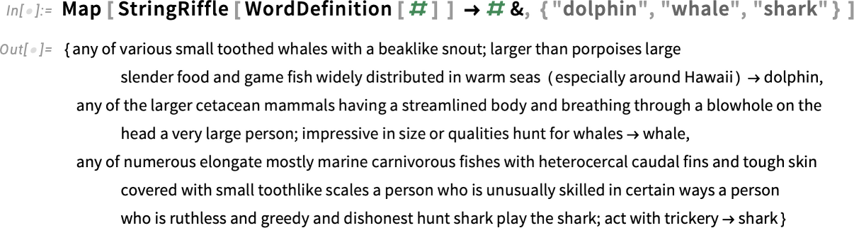
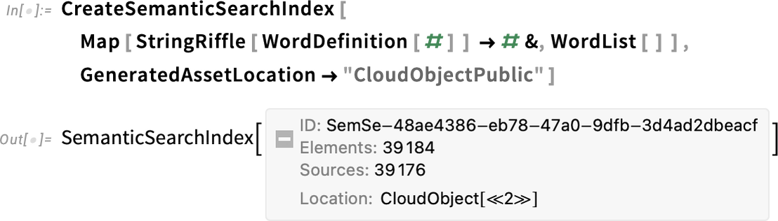
In direct analogy to CreateSearchIndex for TextSearch, there’s now a CreateSemanticSearchIndex for SemanticSearch. Let’s do a tiny example to see how it works. Essentially we’re going to make an (extremely restricted) “inverse dictionary”. We set up a list of definition ![]() word elements:
word elements:
Now create a semantic search index from this:
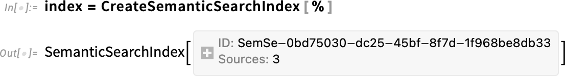
Behind the scenes this is a vector database. But we can access it with SemanticSearch:
And since “whale” is considered closest, it comes first.
What about a more realistic example? Instead of just using 3 words, let’s set up definitions for all words in the dictionary. It takes a little while (like a few minutes) to do the machine learning feature extraction for all the definitions. But in the end you get a new semantic search index:
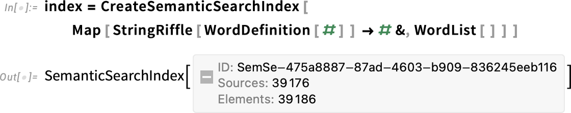
This time it has 39,186 entries—but SemanticSearch picks out the (by default) 10 that it considers closest to what you asked for (and, yes, there’s an archaic definition of “seahorse” as “walrus”):
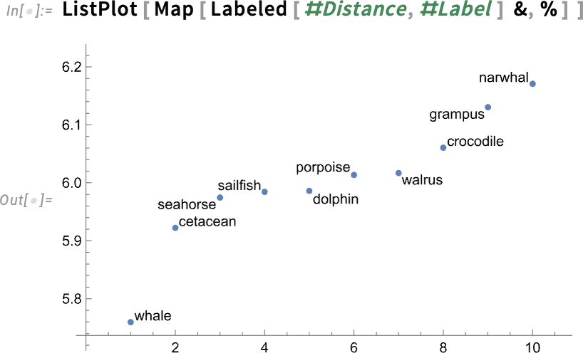
We can see a bit more detail about what’s going on by asking SemanticSearch to explicitly show us distances:

And plotting these we can see that “whale” is the winner by a decent margin:
One subtlety when dealing with semantic search indices is where to store them. When they’re sufficiently small, you can store them directly in memory, or in a notebook. But usually you’ll want to store them in a separate file, and if you want to share an index you’ll want to put this file in the cloud. You can do this either interactively from within a notebook

or programmatically:
And now the SemanticSearchIndex object you have can be used by anyone, with its data being accessed in the cloud.
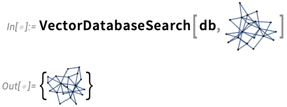
In most cases SemanticSearch will be what you need. But sometimes it’s worthwhile to “go underneath” and directly work with vector databases. Here’s a collection of small vectors:
We can use Nearest to find the nearest vector to one we give:
But we can also do this with a vector database. First we create the database:
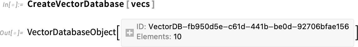
And now we can search for the nearest vector to the one we give:
In this case we get exactly the same answer as from Nearest. But whereas the mission of Nearest is to give us the mathematically precise nearest vector, VectorDatabaseSearch is doing something less precise—but is able to do it for extremely large numbers of vectors that don’t need to be stored directly in memory.
Those vectors can come from anywhere. For example, here they’re coming from extracting features from some images:
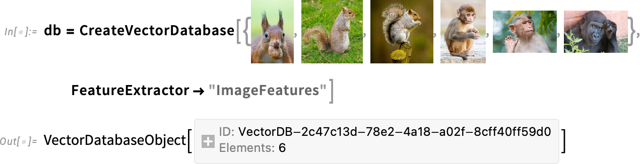
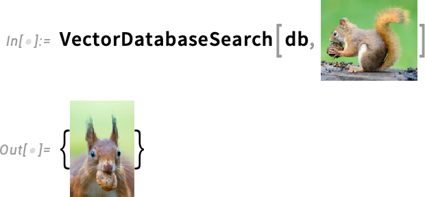
Now let’s say we’ve got a specific image. Then we can search our vector database to get the image whose feature vector is closest to the one for the image we provided:
And, yes, this works for other kinds of objects too:

CreateSemanticSearchIndex and CreateVectorDatabase create vector databases from scratch using data you provide. But—just like with text search indices—an important feature of vector databases is that you can incrementally add to them. So, for example, UpdateSemanticSearchIndex and AddToVectorDatabase let you efficiently add individual entries or lists of entries to vector databases.
In addition to providing capabilities for building (and growing) your own vector databases, there are several pre-built vector databases that are now available in the Wolfram Data Repository:

So now we can use a pre-built vector database of Wolfram Language function documentation to do a semantic search for snippets that are “semantically close” to being about iterating functions:
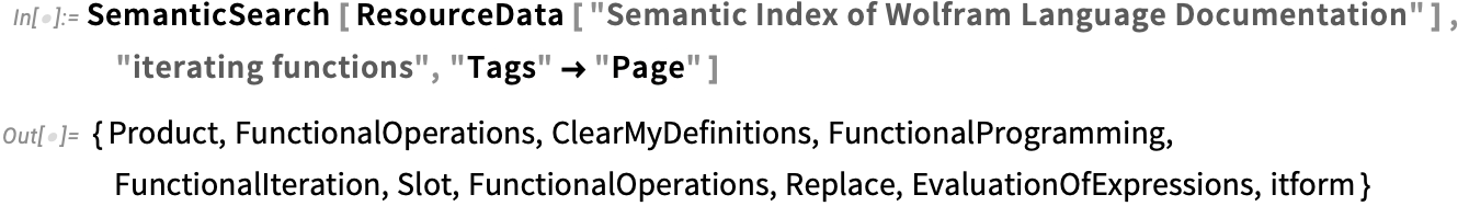
(In the next section, we’ll see how to actually “synthesize a report” based on this.)
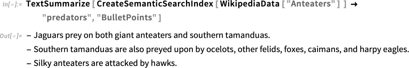
The basic function of SemanticSearch is to determine what “chunks of content” are closest to what you are asking about. But given a semantic search index (AKA vector database) there are also other important things you can do. One of them is to use TextSummarize to ask not for specific chunks but rather for some kind of overall summary of what can be said about a given topic from the content in the semantic search index:
RAGs and Dynamic Prompting for LLMs
How does one tell an LLM what one wants it to do? Fundamentally, one provides a prompt, and then the LLM generates output that “continues” that prompt. Typically the last part of the prompt is the specific question (or whatever) that a user is asking. But before that, there’ll be “pre-prompts” that prime the LLM in various ways to determine how it should respond.
In Version 13.3 in mid-2023 (i.e. a long time ago in the world of LLMs!) we introduced LLMPrompt as a symbolic way to specify a prompt, and we launched the Wolfram Prompt Repository as a broad source for pre-built prompts. Here’s an example of using LLMPrompt with a prompt from the Wolfram Prompt Repository:
In its simplest form, LLMPrompt just adds fixed text to “pre-prompt” the LLM. LLMPrompt is also set up to take arguments that modify the text it’s adding:
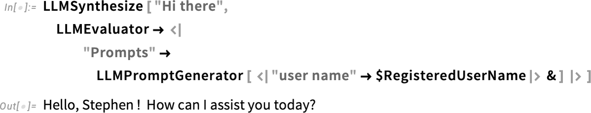
But what if one wants the LLM to be pre-prompted in a way that depends on information that’s only available once the user actually asks their question (like, for example, the text of the question itself)? In Version 14.1 we’re adding LLMPromptGenerator to dynamically generate pre-prompts. And it turns out that this kind of “dynamic prompting” is remarkably powerful, and—particularly together with tool calling—opens up a whole new level of capabilities for LLMs.
For example, we can set up a prompt generator that produces a pre-prompt that gives the registered name of the user, so the LLM can use this information when generating its answer:
Or for example here the prompt generator is producing a pre-prompt about sunrise, sunset and the current time:
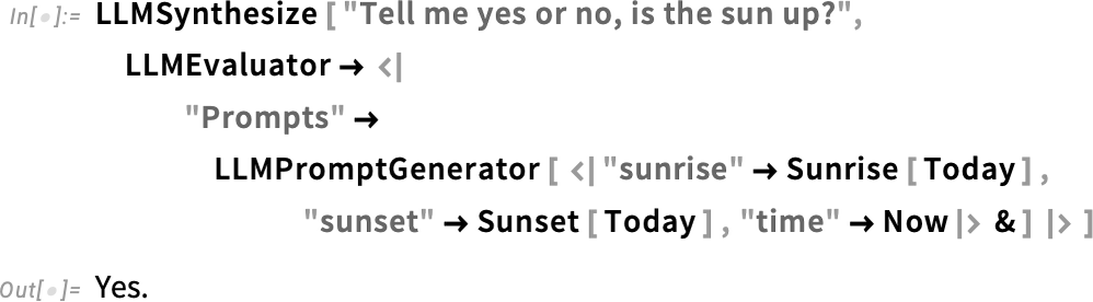
And, yes, if the pre-prompt contains extra information (like about the Moon) the LLM will (probably) ignore it:
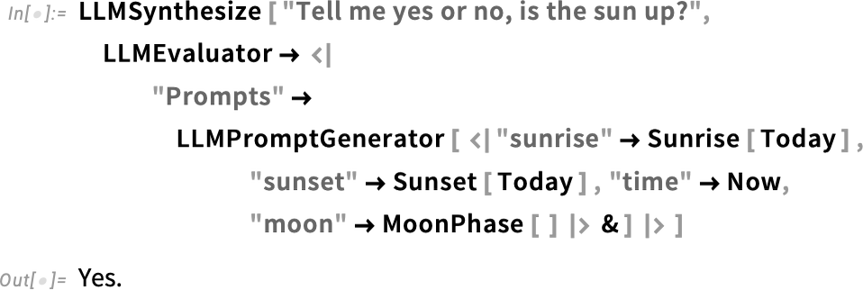
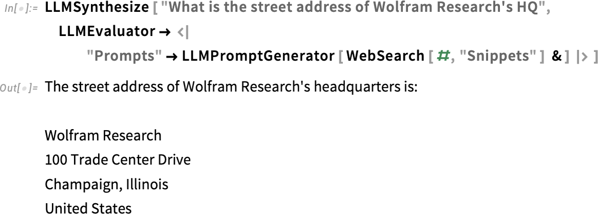
As another example, we can take whatever the user asks, and first do a web search on it, then include as a pre-prompt snippets we get from the web. The result is that we can get answers from the LLM that rely on specific “web knowledge” that we can’t expect will be “known in detail” by the raw LLM:
But often one doesn’t want to just “search at random on the web”; instead one wants to systematically retrieve information from some known source to give as “briefing material” to the LLM to help it in generating its answer. And a typical way to implement this kind of “retrieval-augmented generation (RAG)” is to set up an LLMPromptGenerator that uses the SemanticSearch and vector database capabilities that we introduced in Version 14.1.
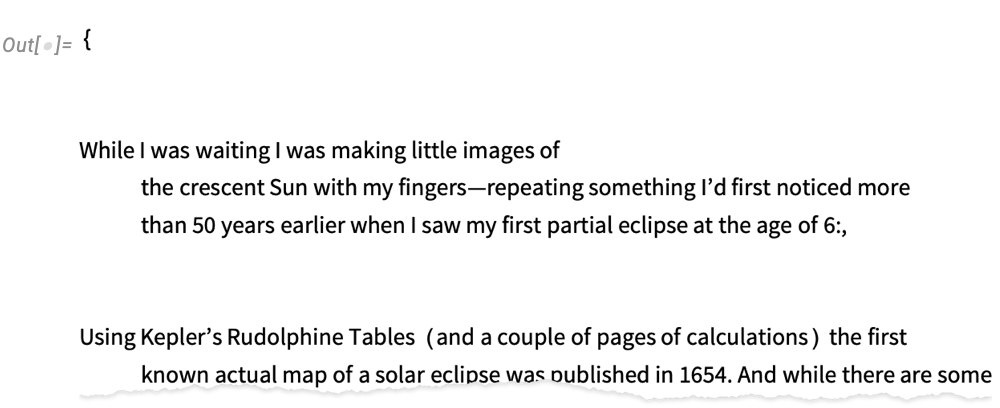
So, for example, here’s a semantic search index generated from my (rather voluminous) writings:
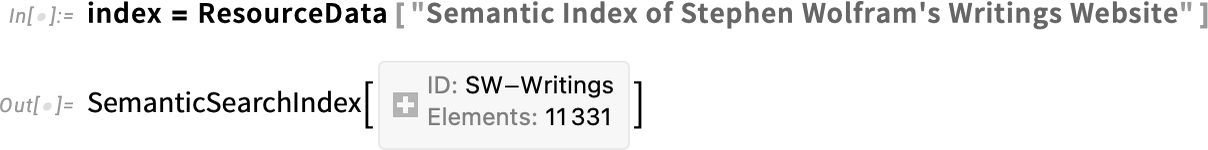
By setting up a prompt generator based on this, I can now ask the LLM “personal questions”:
How did the LLM “know that”? Internally the prompt generator used SemanticSearch to generate a collection of snippets, which the LLM then “trawled through” to produce a specific answer:
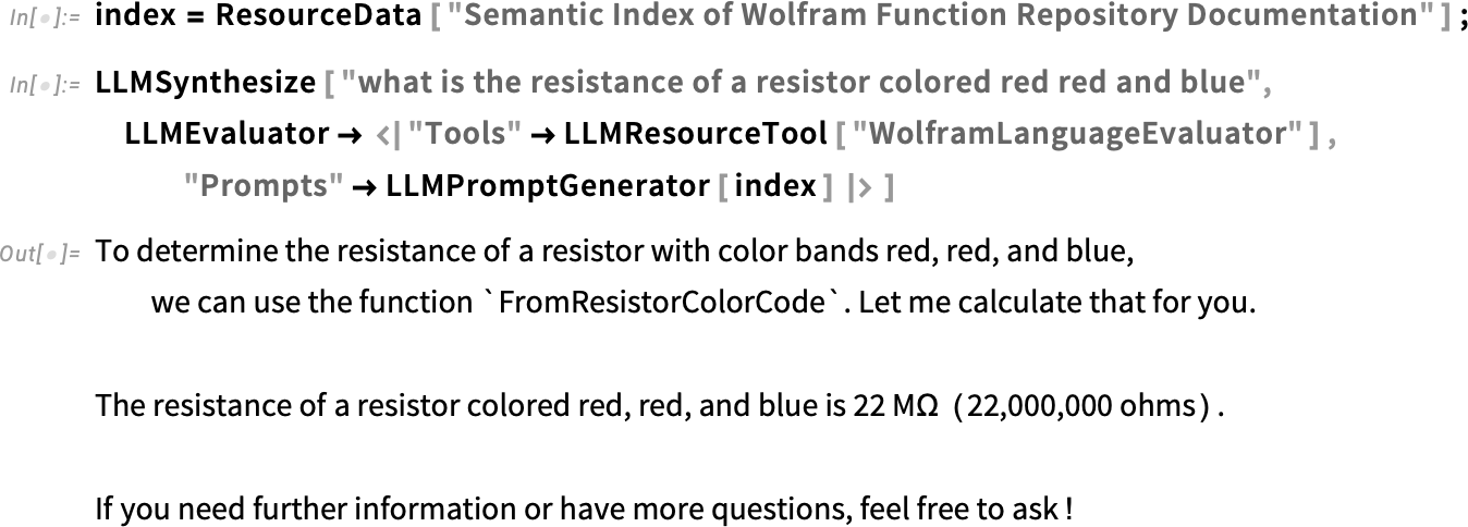
It’s already often very useful just to “retrieve static text” to “brief” the LLM. But even more powerful is to brief the LLM with what it needs to call tools that can do further computation, etc. So, for example, if you want the LLM to write and run Wolfram Language code that uses functions you’ve created, you can do that by having it first “read the documentation” for those functions.
As an example, this uses a prompt generator that uses a semantic search index built from the Wolfram Function Repository:
Connect to Your Favorite LLM
There are now many ways to use LLM functionality from within the Wolfram Language, and Wolfram Notebooks. You can do it programmatically, with LLMFunction, LLMSynthesize, etc. You can do it interactively through Chat Notebooks and related chat capabilities.
But (at least for now) there’s no full-function LLM built directly into the Wolfram Language. So that means that (at least for now) you have to choose your “flavor” of external LLM to power Wolfram Language LLM functionality. And in Version 14.1 we have support for basically all major available foundation-model LLMs.
We’ve made it as straightforward as possible to set up connections to external LLMs. Once you’ve done it, you can select what you want directly in any Chat Notebook

or from your global Preferences:

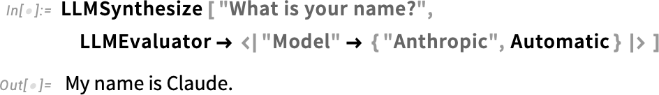
When you’re using a function you specify the “model” (i.e. service and specific model name) as part of the setting for LLMEvaluator:
In general you can use LLMConfiguration to define the whole configuration of an LLM you want to connect to, and you can make a particular configuration your default either interactively using Preferences, or by explicitly setting the value of $LLMEvaluator.
So how do you initially set up a connection to a new LLM? You can do it interactively by pressing Connect in the AI Settings pane of Preferences. Or you can do it programmatically using ServiceConnect:

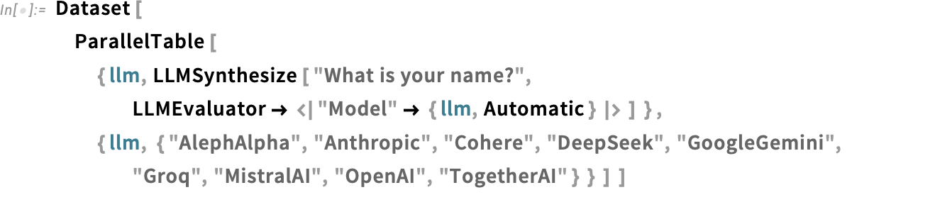
At the “ServiceConnect level” you have very direct access to the features of LLM APIs, though unless you’re studying LLM APIs you probably won’t need to use these. But talking of LLM APIs, one of the things that’s now easy to do with Wolfram Language is to compare LLMs, for example programmatically sending the same question to multiple LLMs:
And in fact we’ve recently started posting weekly results that we get from a full range of LLMs on the task of writing Wolfram Language code (conveniently, the exercises in my book An Elementary Introduction to the Wolfram Language have textual “prompts”, and we have a well-developed system that we’ve used for many years in assessing code for the online course based on the book):

Symbolic Arrays and Their Calculus
I want A to be an n×n matrix. I don’t want to say what its elements are, and I don’t even want to say what n is. I just want to have a way to treat the whole thing symbolically. Well, in Version 14.1 we’ve introduced MatrixSymbol to do that.
A MatrixSymbol has a name (just like an ordinary symbol)—and it has a way to specify its dimensions. We can use it, for example, to set up a symbolic representation for our matrix A:
Hovering over this in a notebook, we’ll get a tooltip that explains what it is:

We can ask for its dimensions as a tensor:
Here’s its inverse, again represented symbolically:
That also has dimensions n×n:
In Version 14.1 you can not only have symbolic matrices, you can also have symbolic vectors and, for that matter, symbolic arrays of any rank. Here’s a length-n symbolic vector (and, yes, we can have a symbolic vector named v that we assign to a symbol v):
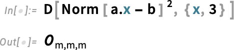
So now we can construct something like the quadratic form:
A classic thing to compute from this is its gradient with respect to the vector ![]() :
:
And actually this is just the same as the “vector derivative”:
If we do a second derivative we get:
What happens if we differentiate ![]() with respect to
with respect to ![]() ? Well, then we get a symbolic identity matrix
? Well, then we get a symbolic identity matrix
which again has dimensions n×n:
![]() is a rank-2 example of a symbolic identity array:
is a rank-2 example of a symbolic identity array:
If we give n an explicit value, we can get an explicit componentwise array:
Let’s say we have a function of ![]() , like Total. Once again we can find the derivative with respect to
, like Total. Once again we can find the derivative with respect to ![]() :
:
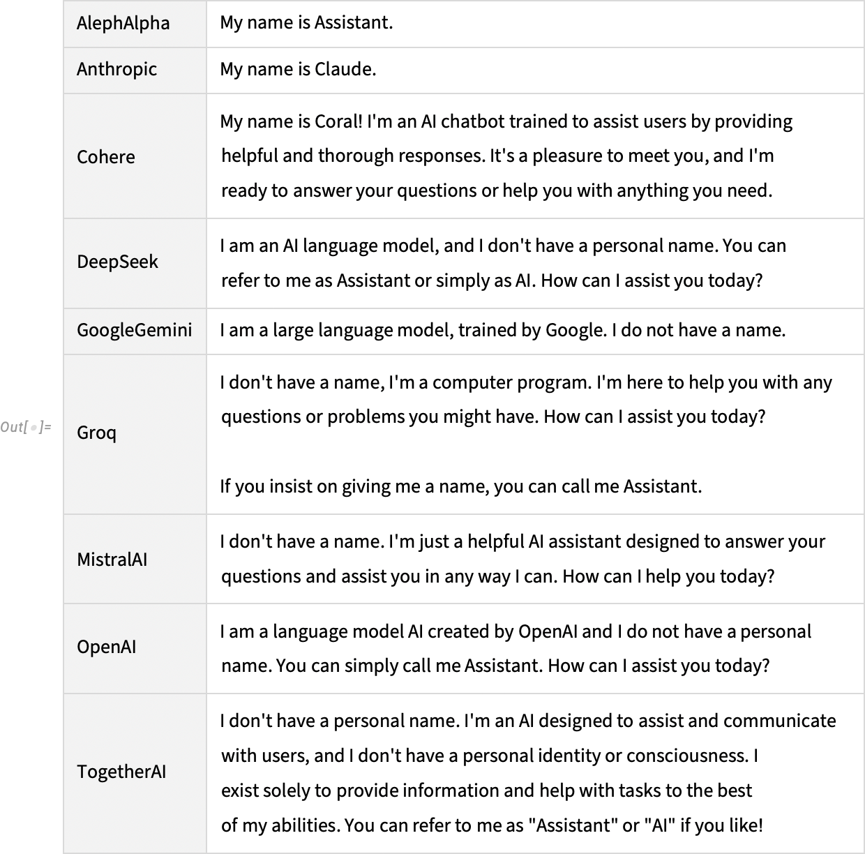
And now we see another symbolic array construct: SymbolicOnesArray:
This is simply an array whose elements are all 1:
Differentiating a second time gives us a SymbolicZerosArray:
Although we’re not defining explicit elements for ![]() , it’s sometimes important to specify, for example, that all the elements are reals:
, it’s sometimes important to specify, for example, that all the elements are reals:
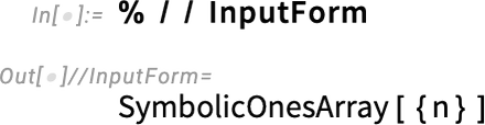
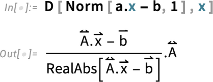
For a vector whose elements are reals, it’s straightforward to find the derivative of the norm:
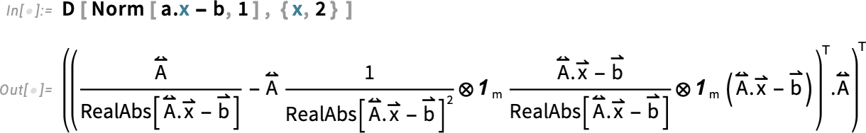
The third derivative, though, is a bit more complicated:
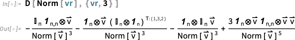
The ⊗ here is TensorProduct, and the T:(1,3,2) represents Transpose[..., {1, 3, 2}].
In the Wolfram Language, a symbol, say s, can stand on its own, and represent a “variable”. It can also appear as a head—as in s[x]—and represent a function. And the same is true for vector and matrix symbols:
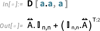
Importantly, the chain rule also works for matrix and vector functions:
Things get a bit trickier when one’s dealing with functions of matrices:
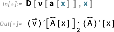
The ![]() here represents ArrayDot[..., ..., 2], which is a generalization of Dot. Given two arrays u and v, Dot will contract the last index of u with the first index of v:
here represents ArrayDot[..., ..., 2], which is a generalization of Dot. Given two arrays u and v, Dot will contract the last index of u with the first index of v:
ArrayDot[u, v, n], on the other hand, contracts the last n indices of u with the first n of v.
But now in this particular example all the indices get “contracted out”:
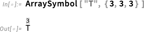
We’ve talked about symbolic vectors and matrices. But—needless to say—what we have is completely general, and will work for arrays of any rank. Here’s an example of a p×q×r array:
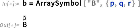
The overscript ![]() indicates that this is an array of rank 3.
indicates that this is an array of rank 3.
When one takes derivatives, it’s very easy to end up with high-rank arrays. Here’s the result of differentiating with respect to a matrix:
![]() is a rank-4 n×n×n×n identity array.
is a rank-4 n×n×n×n identity array.
When one’s dealing with higher-rank objects, there’s one more construct that appears—that we call SymbolicDeltaProductArray. Let’s set up a rank-3 array with dimensions 3×3×3:
Now let’s compute a derivative:
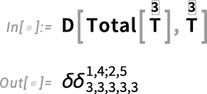
The result is a rank-5 array that’s effectively a combination of two KroneckerDelta objects for indices 1,4 and 2,5, respectively:
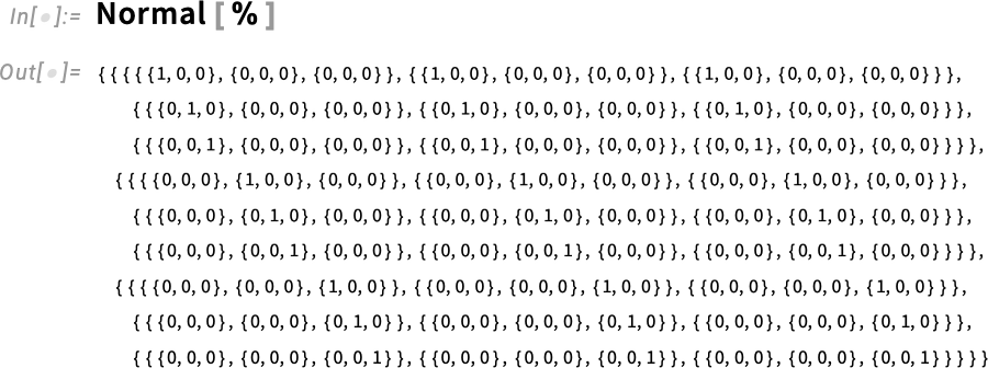
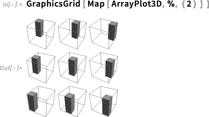
We can visualize this with ArrayPlot3D:
The most common way to deal with arrays in the Wolfram Language has always been in terms of explicit lists of elements. And in this representation it’s extremely convenient that operations are normally done elementwise:
Non-lists are then by default treated as scalars—and for example here added into every element:
But now there’s something new, namely symbolic arrays—which in effect implicitly contain multiple list elements, and thus can’t be “added into every element”:
This is what happens when we have an “ordinary scalar” together with a symbolic vector:
How does this work? “Under the hood” there’s a new attribute NonThreadable which specifies that certain heads (like ArraySymbol) shouldn’t be threaded by Listable functions (like Plus).
By the way, ever since Version 9 a dozen years ago we’ve had a limited mechanism for assuming that symbols represent vectors, matrices or arrays—and now that mechanism interoperates with all our new symbolic array functionality:
When you’re doing explicit computations there’s often no choice but to deal directly with individual array elements. But it turns out that there are all sorts of situations where it’s possible to work instead in terms of “whole” vectors, matrices, etc. And indeed in the literature of fields like machine learning, optimization, statistics and control theory, it’s become quite routine to write down formulas in terms of symbolic vectors, matrices, etc. And what Version 14.1 now adds is a streamlined way to compute in terms of these symbolic array constructs.
The results are often very elegant. So, for example, here’s how one might set up a general linear least-squares problem using our new symbolic array constructs. First we define a symbolic n×m matrix A, and symbolic vectors b and x:
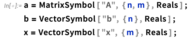
Our goal is to find a vector ![]() that minimizes
that minimizes ![]() . And with our definitions we can now immediately write down this quantity:
. And with our definitions we can now immediately write down this quantity:
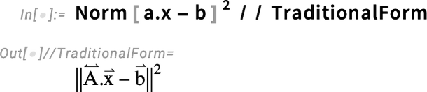
To extremize it, we compute its derivative
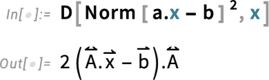
and to ensure we get a minimum, we compute the second derivative:
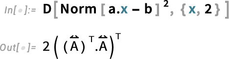
These are standard textbook formulas, but the cool thing is that in Version 14.1 we’re now in a position to generate them completely automatically. By the way, if we take another derivative, the result will be a zero tensor:
We can look at other norms too:
Binomials and Pitchforks: Navigating Mathematical Conventions
Binomial coefficients have been around for at least a thousand years, and one might not have thought there could possibly be anything shocking or controversial about them anymore (notwithstanding the fictional Treatise on the Binomial Theorem by Sherlock Holmes’s nemesis Professor Moriarty). But in fact we have recently been mired in an intense debate about binomial coefficients—which has caused us in Version 14.1 to introduce a new function PascalBinomial alongside our existing Binomial.
When one’s dealing with positive integer arguments, there’s no issue with binomials. And even when one extends to generic complex arguments, there’s again a unique way to do this. But negative integer arguments are a special degenerate case. And that’s where there’s trouble—because there are two different definitions that have historically been used.
In early versions of Mathematica, we picked one of these definitions. But over time we realized that it led to some subtle inconsistencies, and so for Version 7—in 2008—we changed to the other definition. Some of our users were happy with the change, but some were definitely not. A notable (vociferous) example was my friend Don Knuth, who has written several well-known books that make use of binomial coefficients—always choosing what amounts to our pre-2008 definition.
So what could we do about this? For a while we thought about adding an option to Binomial, but to do this would have broken our normal conventions for mathematical functions. And somehow we kept on thinking that there was ultimately a “right answer” to how binomial coefficients should be defined. But after a lot of discussion—and historical research—we finally concluded that since at least before 1950 there have just been two possible definitions, each with their own advantages and disadvantages, with no obvious “winner”. And so in Version 14.1 we decided just to introduce a new function PascalBinomial to cover the “other definition”.
And—though at first it might not seem like much—here’s a big difference between Binomial and PascalBinomial:
Part of why things get complicated is the relation to symbolic computation. Binomial has a symbolic simplification rule, valid for any n:
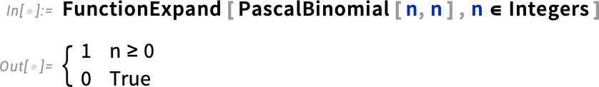
But there isn’t a corresponding generic simplification rule for PascalBinomial:
FunctionExpand shows us the more nuanced result in this case:
To see a bit more of what’s going on, we can compute arrays of nonzero results for Binomial and PascalBinomial:
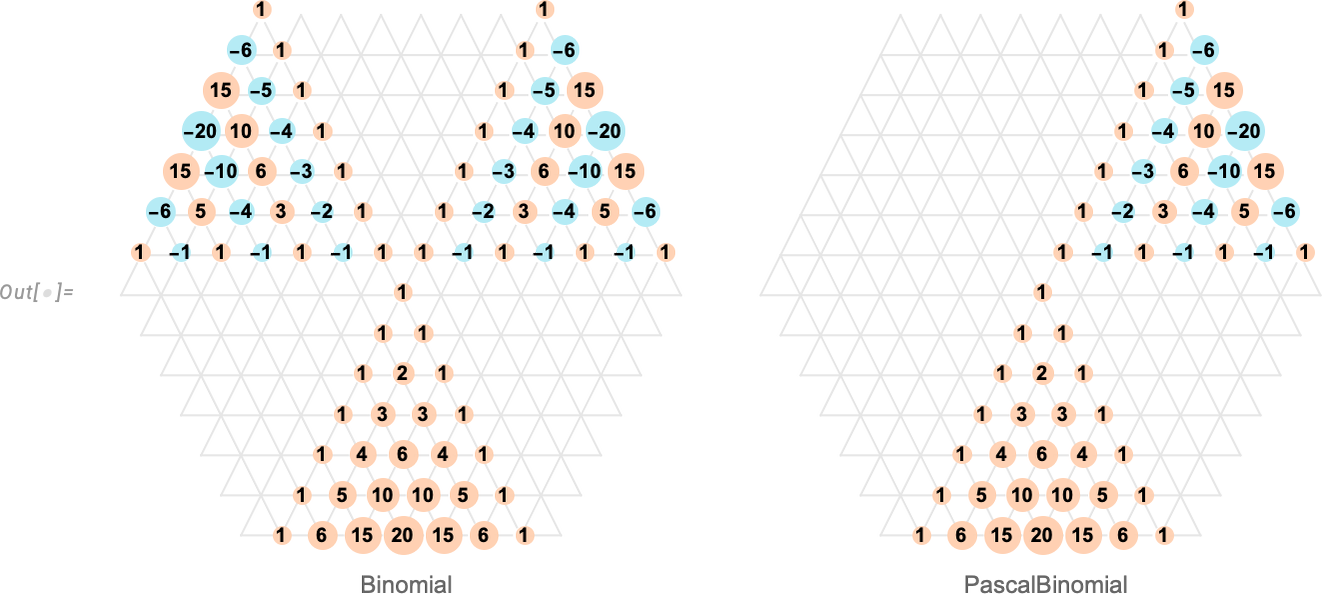
Binomial[n, k] has the “nice feature” that it’s symmetric in k even when n < 0. But this has the “bad consequence” that Pascal’s identity (that says a particular binomial coefficient is the sum of two coefficients “above it”) isn’t always true. PascalBinomial, on the other hand, always satisfies the identity, and it’s in recognition of this that we put “Pascal” in its name.
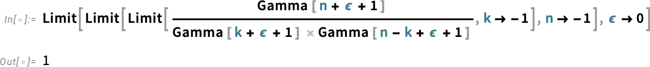
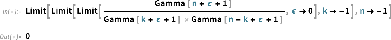
And, yes, this is all quite subtle. And, remember, the differences between Binomial and PascalBinomial only show up at negative integer values. Away from such values, they’re both given by the same expression, involving gamma functions. But at negative integer values, they correspond to different limits, respectively:
The story of Binomial and PascalBinomial is a complicated one that mainly affects only the upper reaches of discrete mathematics. But there’s another, much more elementary convention that we’ve also tackled in Version 14.1: the convention of what the arguments of trigonometric functions mean.
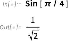
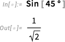
We’ve always taken the “fundamentally mathematical” point of view that the x in Sin[x] is in radians:
You’ve always been able to explicitly give the argument in degrees (using Degree—or after Version 3 in 1996—using °):
But a different convention would just say that the argument to Sin should always be interpreted as being in degrees, even if it’s just a plain number. Calculators would often have a physical switch that globally toggles to this convention. And while that might be OK if you are just doing a small calculation and can physically see the switch, nothing like that would make any sense at all in our system. But still, particularly in elementary mathematics, one might want a “degrees version” of trigonometric functions. And in Version 14.1 we’ve introduced these:
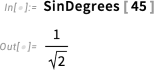
One might think this was somewhat trivial. But what’s nontrivial is that the “degrees trigonometric functions” are consistently integrated throughout the system. Here, for example, is the period in SinDegrees:
You can take the integral as well

and the messiness of this form shows why for more than three decades we’ve just dealt with Sin[x] and radians.
Fixed Points and Stability for Differential and Difference Equations
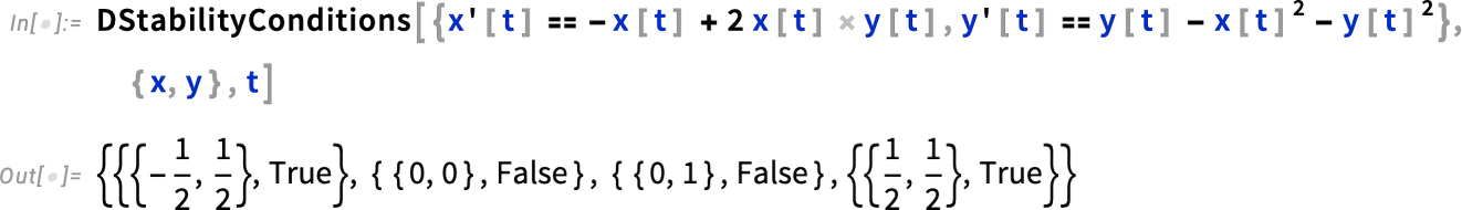
All sorts of differential equations have the feature that their solutions exhibit fixed points. It’s always in principle been possible to find these by looking for points where derivatives vanish. But in Version 14.1 we now have a general, robust function that takes the same form of input as DSolve and finds all fixed points:
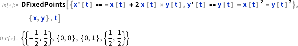
Here’s a stream plot of the solutions to our equations, together with the fixed points we’ve found:
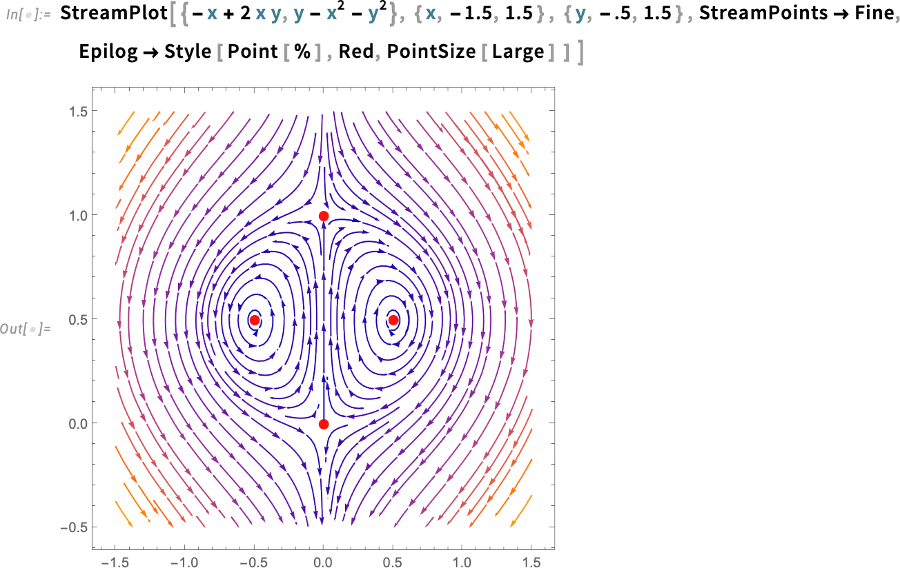
And we can see that there are two different kinds of fixed points here. The ones on the left and right are “stable” in the sense that solutions that start near them always stay near them. But it’s a different story for the fixed points at the top and bottom; for these, solutions that start nearby can diverge. The function DStabilityConditions computes fixed points, and specifies whether they are stable or not:
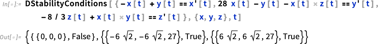
As another example, here are the Lorenz equations, which have one unstable fixed point, and two stable ones:
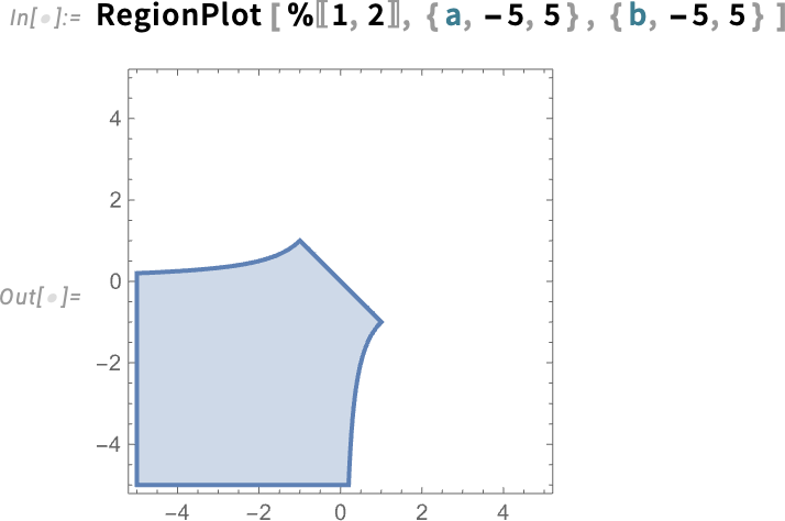
If your equations have parameters, their stability fixed points can depend on those parameters:

Extracting the conditions here, we can now plot the region of parameter space where this fixed point is stable:
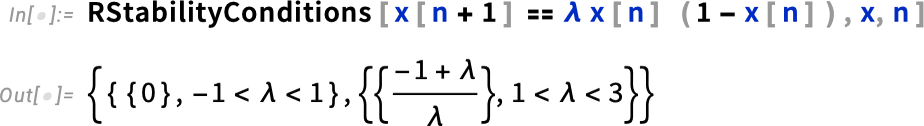
This kind of stability analysis is important in all sorts of fields, including dynamical systems theory, control theory, celestial mechanics and computational ecology.
And just as one can find fixed points and do stability analysis for differential equations, one can also do it for difference equations—and this is important for discrete dynamical systems, digital control systems, and for iterative numerical algorithms. Here’s a classic example in Version 14.1 for the logistic map:
The Steady Advance of PDEs
Five years ago—in Version 11.3—we introduced our framework for symbolically representing physical systems using PDEs. And in every version since we’ve been steadily adding more and more capabilities. At this point we’ve now covered the basics of heat transfer, mass transport, acoustics, solid mechanics, fluid mechanics, electromagnetics and (one-particle) quantum mechanics. And with our underlying symbolic framework, it’s easy to mix components of all these different kinds.
Our goal now is to progressively cover what’s needed for more and more kinds of applications. So in Version 14.1 we’re adding von Mises stress analysis for solid mechanics, electric current density models for electromagnetics and anisotropic effective masses for quantum mechanics.
So as an example of what’s now possible, here’s a piece of geometry representing a spiral inductor of the kind that might be used in a modern MEMS device:

Let’s define our variables—voltage and position:
And let’s specify parameters—here just that the material we’re going to deal with is copper:
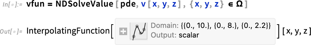
Now we’re in a position to set up the PDE for this system, making use of the new constructs ElectricCurrentPDEComponent and ElectricCurrentDensityValue:

All it takes to solve this PDE for the voltage is then:
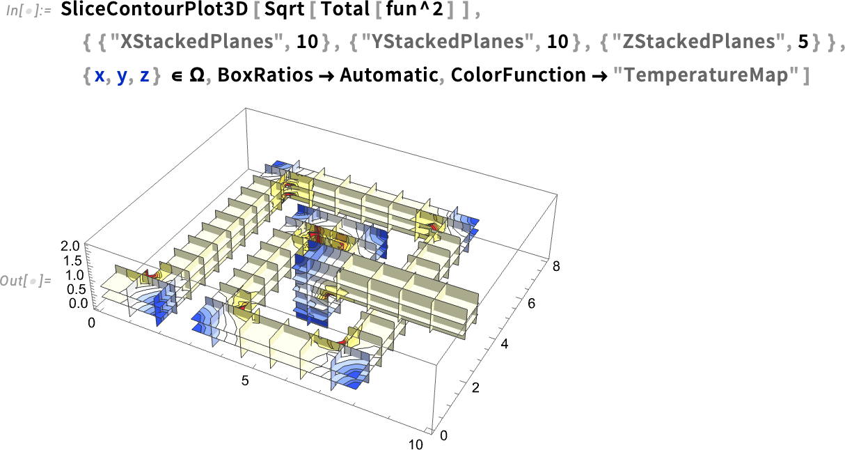
From the voltage we can compute the current density
and then plot it (and, yes, the current tends to avoid the corners):
Symbolic Biomolecules and Their Visualization
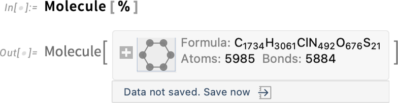
Ever since Version 12.2 we’ve had the ability to represent and manipulate bio sequences of the kind that appear in DNA, RNA and proteins. We’ve also been able to do things like import PDB (Protein Data Bank) files and generate graphics from them. But now in Version 14.1 we’re adding a symbolic BioMolecule construct, to represent the full structure of biomolecules:
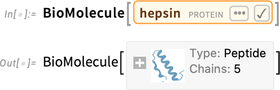
Ultimately this is “just a molecule” (and in this case its data is so big it’s not by default stored locally in your notebook):
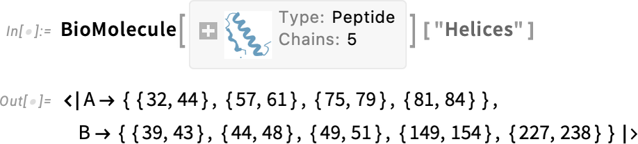
But what BioMolecule does is also to capture the “higher-order structure” of the molecule, for example how it’s built up from distinct chains, where structures like α-helices occur in these, and so on. For example, here are the two (bio sequence) chains that appear in this case:
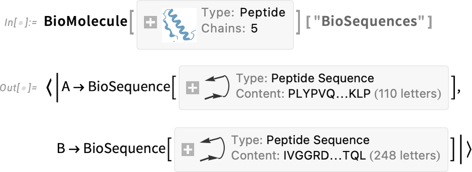
And here are where the α-helices occur:
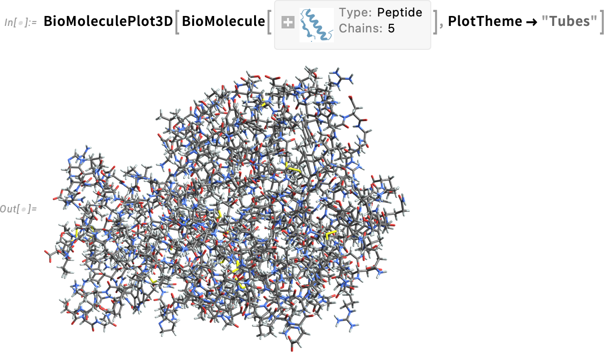
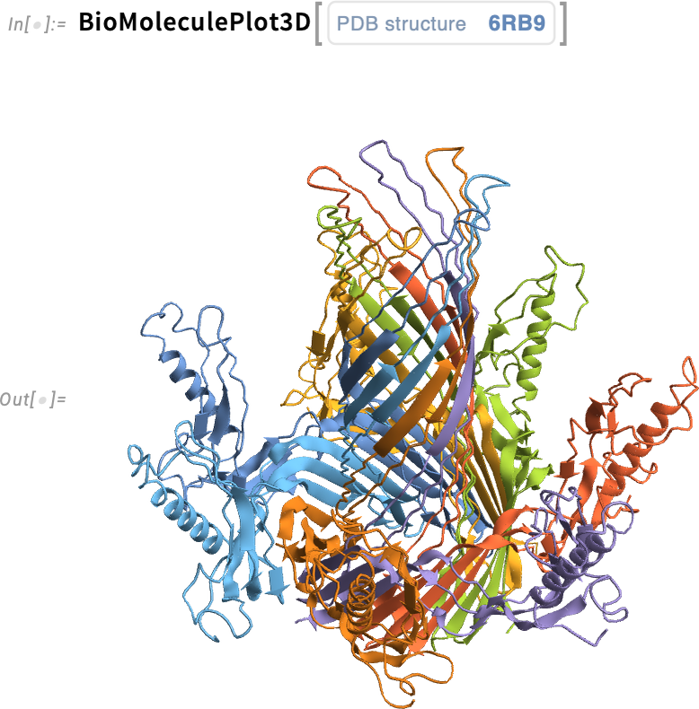
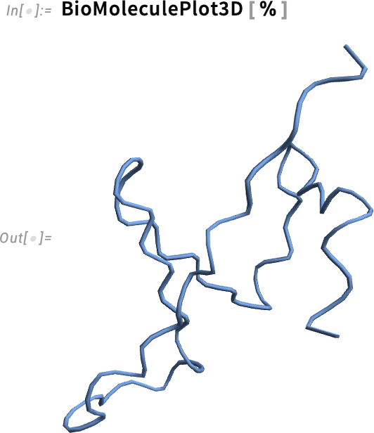
What about visualization? Well, there’s BioMoleculePlot3D for that:
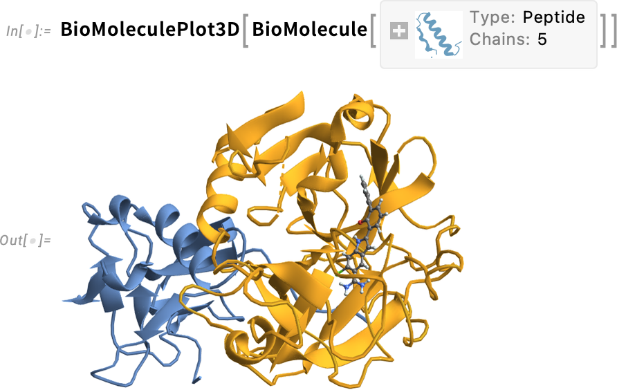
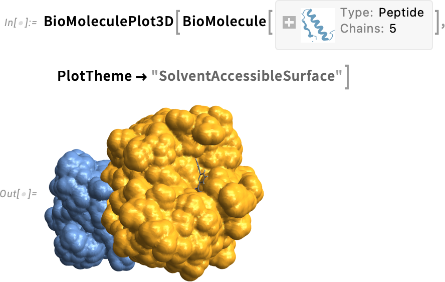
There are different “themes” you can use for this:
Here’s a raw-atom-level view:
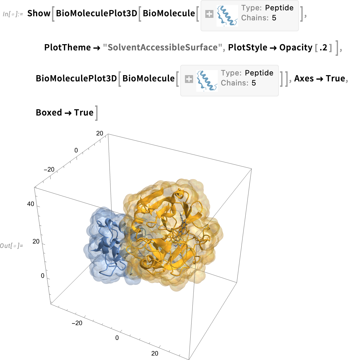
You can combine the views—and for example add coordinate values (specified in angstroms):
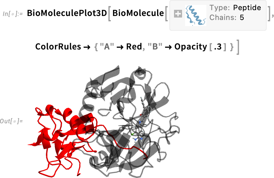
You can also specify “color rules” that define how particular parts of the biomolecule should be rendered:
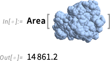
But the structure here isn’t just something you can make graphics out of; it’s also something you can compute with. For example, here’s a geometric region formed from the biomolecule:
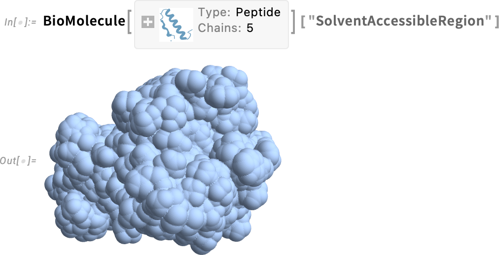
And this computes its surface area (in square angstroms):
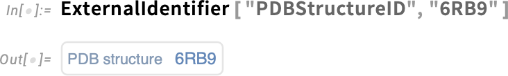
The Wolfram Language has built-in data on a certain number of proteins. But you can get data on many more proteins from external sources—specifying them with external identifiers:
When you get a protein—say from an external source—it’ll often come with a 3D structure specified, for example as deduced from experimental measurements. But even without that, Version 14.1 will attempt to find at least an approximate structure—by using machine-learning-based protein-folding methods. As an example, here’s a random bio sequence:
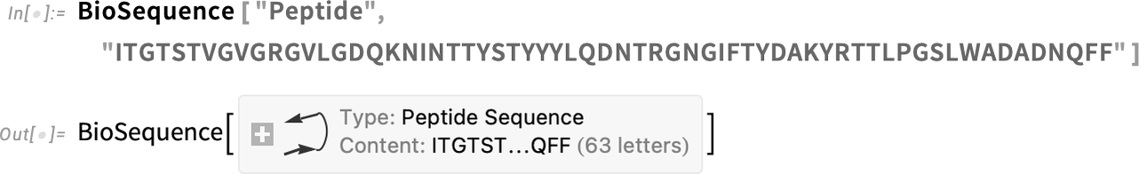
If you make a BioMolecule out of this, a “predicted” 3D structure will be generated:

Here’s a visualization of this structure—though more work would be needed to determine how it’s related to what one might actually observe experimentally:
Optimizing Neural Nets for GPUs and NPUs
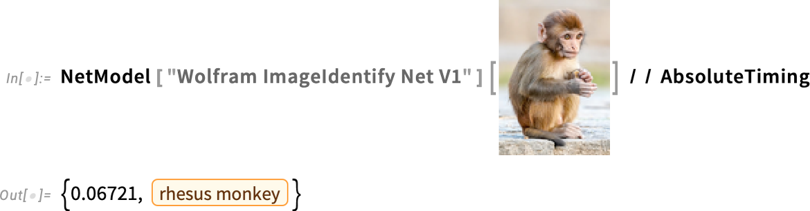
Many computers now come with GPU and NPU hardware accelerators for machine learning, and in Version 14.1 we’ve added more support for these. Specifically, on macOS (Apple Silicon) and Windows machines, built-in functions like ImageIdentify and SpeechRecognize now automatically use CoreML (Neural Engine) and DirectML capabilities—and the result is typically 2X to 10X faster performance.
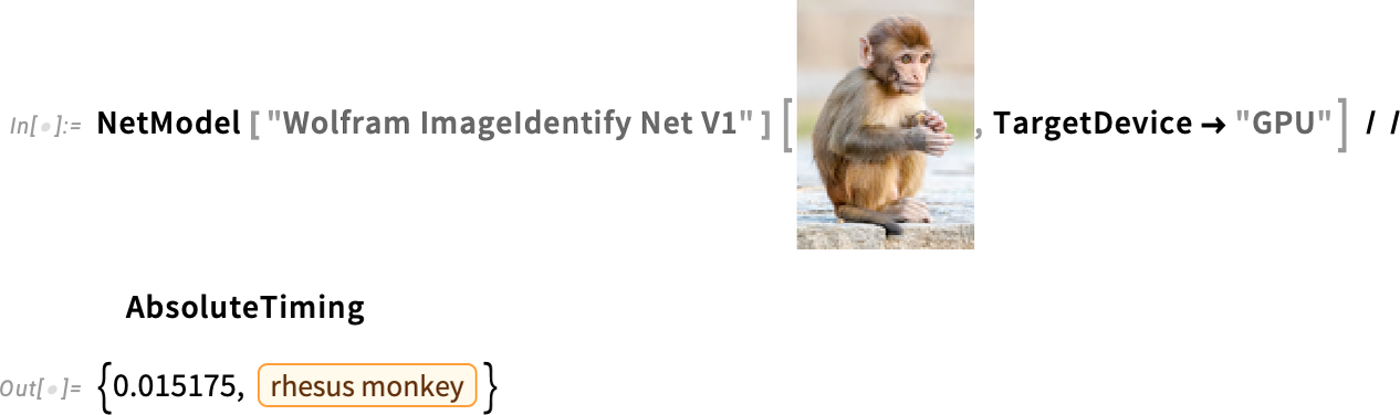
We’ve always supported explicit CUDA GPU acceleration, for both training and inference. But in Version 14.1 we now support CoreML and DirectML acceleration for inference tasks with explicitly specified neural nets. But whereas this acceleration is now the default for built-in machine-learning-based functions, for explicitly specified models the default isn’t yet the default.
So, for example, this doesn’t use GPU acceleration:
But you can explicitly request it—and then (assuming all features of the model can be accelerated) things will typically run significantly faster:
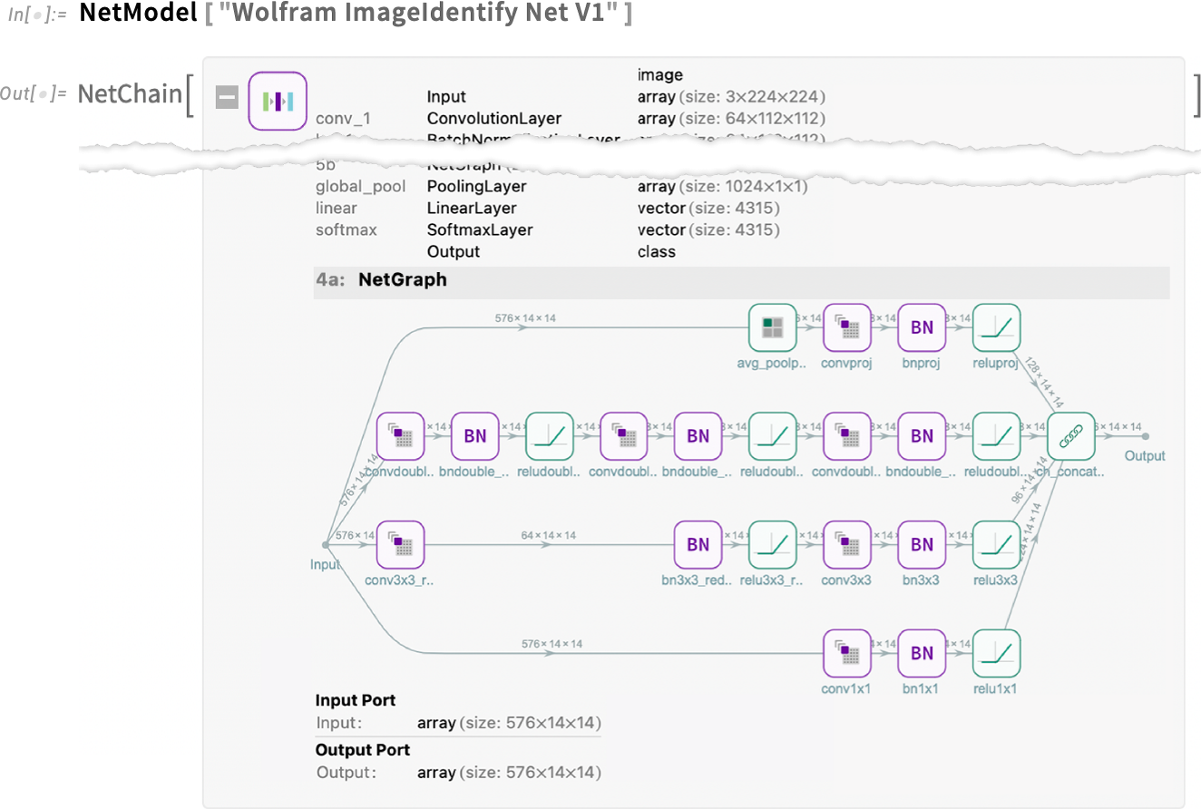
We’re continually sprucing up our infrastructure for machine learning. And as part of that, in Version 14.1 we’ve enhanced our diagrams for neural nets to make layers more visually distinct—and to immediately produce diagrams suitable for publication:
The Statistics of Dates
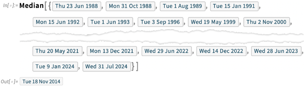
We’ve been releasing versions of what’s now the Wolfram Language for 36 years. And looking at that whole collection of release dates, we can ask statistical questions. Like “What’s the median date for all the releases so far?” Well, in Version 14.1 there’s a direct way to answer that—because statistical functions like Median now just immediately work on dates:
What if we ask about all 7000 or so functions in the Wolfram Language? Here’s a histogram of when they were introduced:
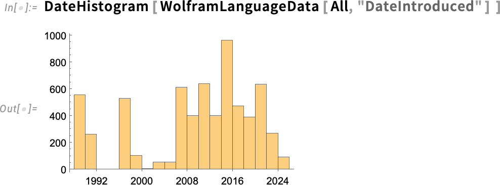
And now we can compute the median, showing quantitatively that, yes, Wolfram Language development has speeded up:
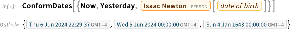
Dates are a bit like numbers, but not quite. For example, their “zero” shifts around depending on the calendar. And their granularity is more complicated than precision for numbers. In addition, a single date can have multiple different representations (say in different calendars or with different granularities). But it nevertheless turns out to be possible to define many kinds of statistics for dates. To understand these statistics—and to compute them—it’s typically convenient to make one’s whole collection of dates have the same form. And in Version 14.1 this can be achieved with the new function ConformDates (which here converts all dates to the format of the first one listed):
By the way, in Version 14.1 the whole pipeline for handling dates (and times) has been dramatically speeded up, most notably conversion from strings, as needed in the import of dates.
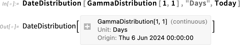
The concept of doing statistics on dates introduces another new idea: date (and time) distributions. And in Version 14.1 there are two new functions DateDistribution and TimeDistribution for defining such distributions. Unlike for numerical (or quantity) distributions, date and time distributions require the specification of an origin, like Today, as well as of a scale, like "Days":
But given this symbolic specification, we can now do operations just like for any other distribution, say generating some random variates:
Building Videos with Programs
Introduced in Version 6 back in 2007, Manipulate provides an immediate way to create an interactive “manipulable” interface. And it’s been possible for a long time to export Manipulate objects to video. But just what should happen in the video? What sliders should move in what way? In Version 12.3 we introduced AnimationVideo to let you make a video in which one parameter is changing with time. But now in Version 14.1 we have ManipulateVideo which lets you create a video in which many parameters can be varied simultaneously. One way to specify what you want is to say for each parameter what value it should get at a sequence of times (by default measured in seconds from the beginning of the video). ManipulateVideo then produces a smooth video by interpolating between these values:
(An alternative is to specify complete “keyframes” by giving operations to be done at particular times.)
ManipulateVideo in a sense provides a “holistic” way to create a video by controlling a Manipulate. And in the last several versions we’ve introduced many functions for creating videos from “existing structures” (for example FrameListVideo assembles a video from a list of frames). But sometimes you want to build up videos one frame at a time. And in Version 14.1 we’ve introduced SowVideo and ReapVideo for doing this. They’re basically the analog of Sow and Reap for video frames. SowVideo will “sow” one or more frames, and all frames you sow will then be collected and assembled into a video by ReapVideo:
One common application of SowVideo/ReapVideo is to assemble a video from frames that are programmatically picked out by some criterion from some other video. So, for example, this “sows” frames that contain a bird, then “reaps” them to assemble a new video.
Another way to programmatically create one video from another is to build up a new video by progressively “folding in” frames from an existing video—which is what the new function VideoFrameFold does:
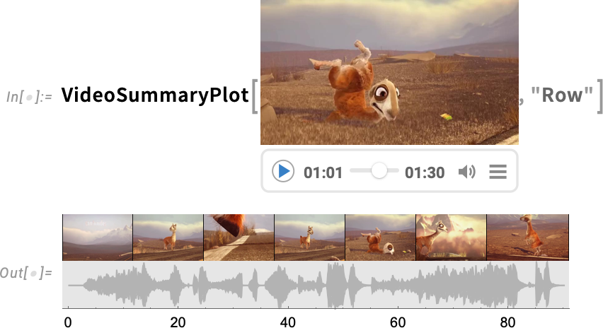
Version 14.1 also has a variety of new “convenience functions” for dealing with videos. One example is VideoSummaryPlot which generates various “at-a-glance” summaries of videos (and their audio):

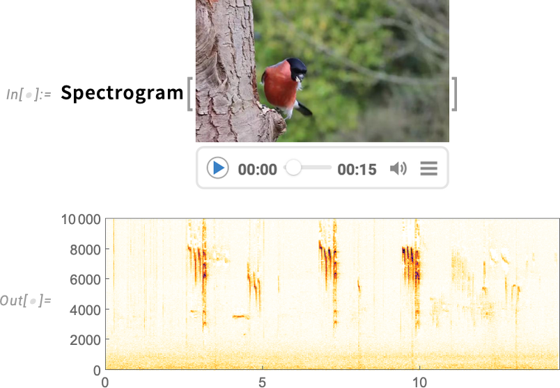
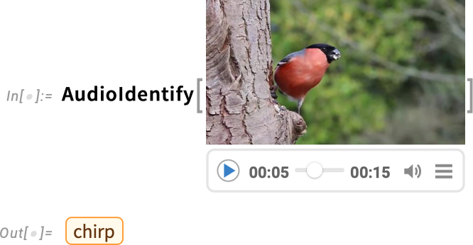
Another new feature in Version 14.1 is the ability to apply audio processing functions directly to videos:
And, yes, it’s a bird:
Optimizing the Speech Recognition Workflow
We first introduced SpeechRecognize in 2019 in Version 12.0. And now in Version 14.1 SpeechRecognize is getting a makeover.
The most dramatic change is speed. In the past, SpeechRecognize would typically take at least as long to recognize a piece of speech as the duration of the speech itself. But now in Version 14.1, SpeechRecognize runs many tens of times faster, so you can recognize speech much faster than real time.
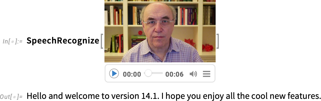
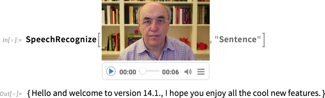
And what’s more, SpeechRecognize now produces full, written text, complete with capitalization, punctuation, etc. So here, for example, is a transcription of a little video:
There’s also a new function, VideoTranscribe, that will take a video, transcribe its audio, and insert the transcription back into the subtitle track of the video.
And, by the way, SpeechRecognize runs entirely locally on your computer, without having to access a server (except maybe for updates to the neural net it’s using).
In the past SpeechRecognize could only handle English. In Version 14.1 it can handle 100 languages—and can automatically produce translated transcriptions. (By default it produces transcriptions in the language you’ve specified with $Language.) And if you want to identify what language a piece of audio is in, LanguageIdentify now works directly on audio.
SpeechRecognize by default produces a single string of text. But it now also has the option to break up its results into a list, say of sentences:
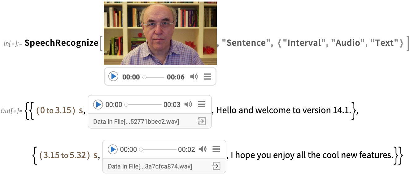
And in addition to producing a transcription, SpeechRecognize can give time intervals or audio fragments for each element:
Historical Geography Becomes Computable
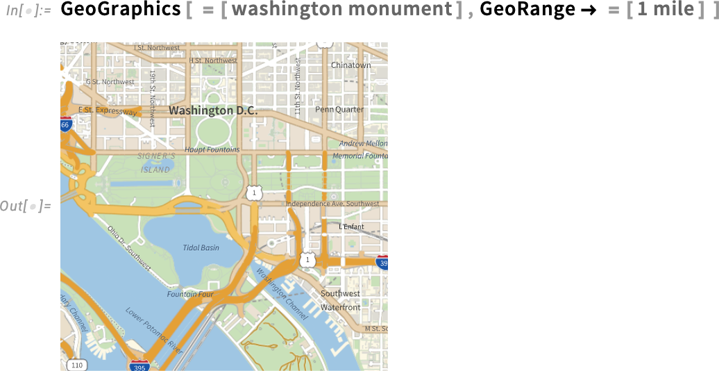
History is complicated. But that doesn’t mean there isn’t much that can be made computable about it. And in Version 14.1 we’re taking a major step forward in making historical geography computable. We’ve had extensive geographic computation capabilities in the Wolfram Language for well over a decade. And in Version 14.1 we’re extending that to historical geography.
So now you can not only ask for a map of where the current country of Italy is, you can also ask to make a map of the Roman Empire in 100 AD:

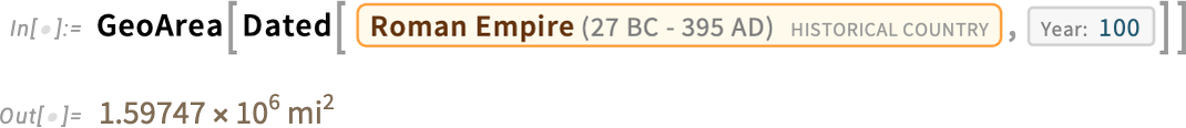
And “the Roman Empire in 100 AD” is now a computable entity. So you can ask for example what its approximate area was:
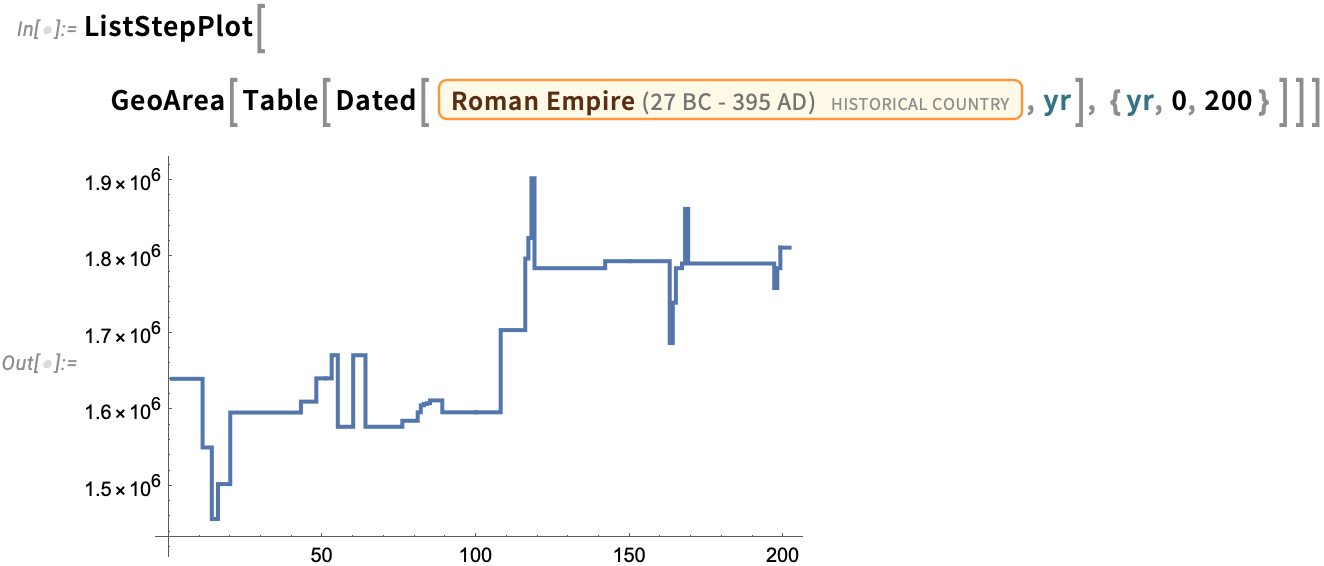
And you can even make a plot of how the area of the Roman Empire changed over the period from 0 AD to 200 AD:
We’ve been building our knowledgebase of historical geography for many years. Of course, country borders may be disputed, and—particularly in the more distant past—may not have been well defined. But by now we’ve accumulated computable data on basically all of the few thousand known historical countries. Still—with history being complicated—it’s not surprising that there are all sorts of often subtle issues.
Let’s start by asking what historical countries the location that’s now Mexico City has been in. GeoIdentify gives the answer:
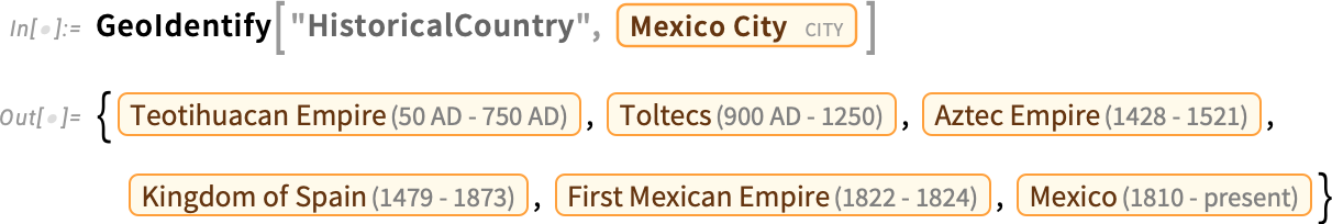
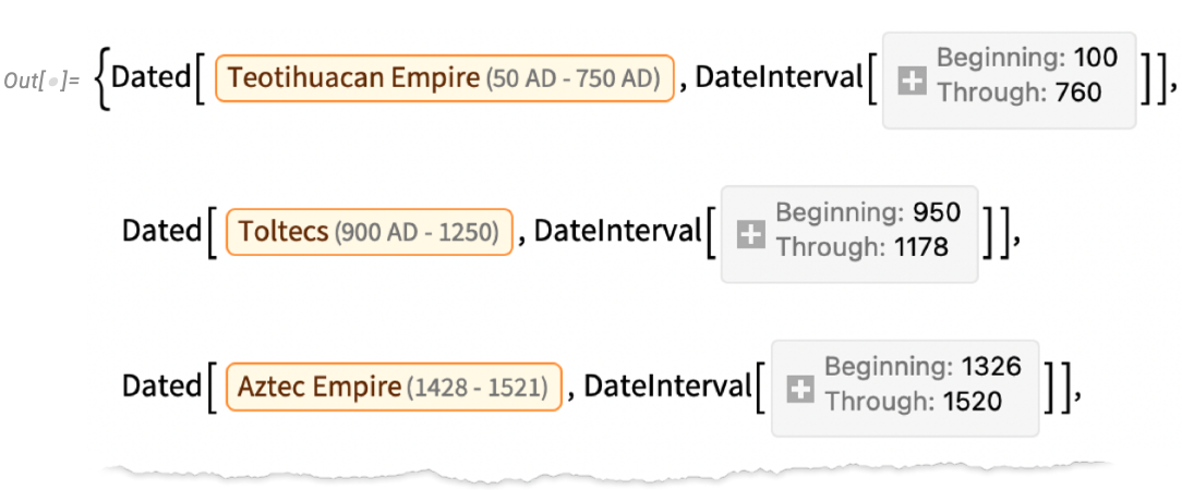
And already we see subtlety. For example, our historical country entities are labeled by their overall beginning and ending dates. But most of them covered Mexico City only for part of their existence. And here we can see what’s going on:
Often there’s subtlety in identifying what should count as a “different country”. If there was just an “acquisition” or a small “change of management” maybe it’s still the same country. But if there was a “dramatic reorganization”, maybe it’s a different country. Sometimes the names of countries (if they even had official names) give clues. But in general it’s taken lots of case-by-case curation, trying to follow the typical conventions used by historians of particular times and places.
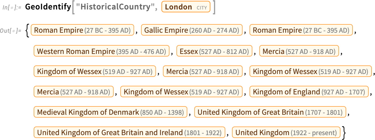
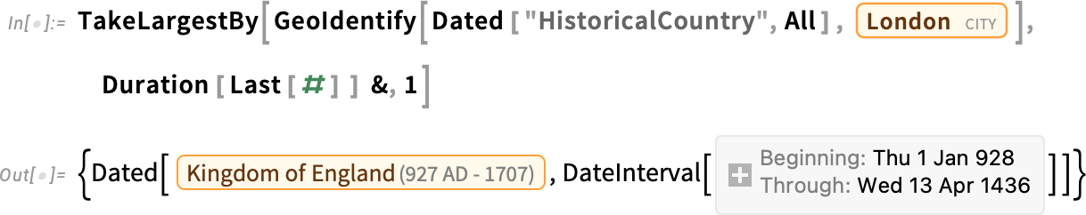
For London we see several “close-but-we-consider-it-a-different-country” issues—along with various confusing repeated conquerings and reconquerings:
Here’s a timeline plot of the countries that have contained London:
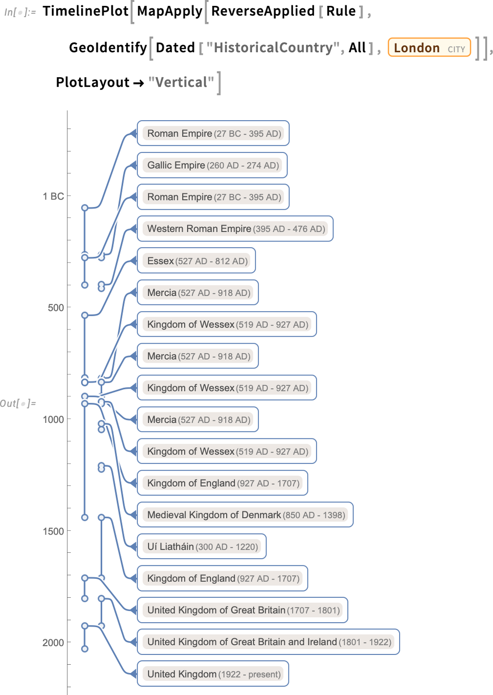
And because everything is computable, it’s easy to identify the longest contiguous segment here:
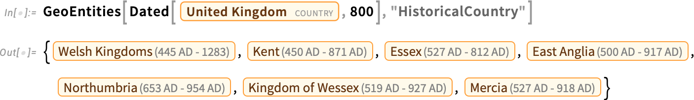
GeoIdentify can tell us what entities something like a city is inside. GeoEntities, on the other hand, can tell us what entities are inside something like a country. So, for example, this tells us what historical countries were inside (or at least overlapped with) the current boundaries of the UK in 800 AD:
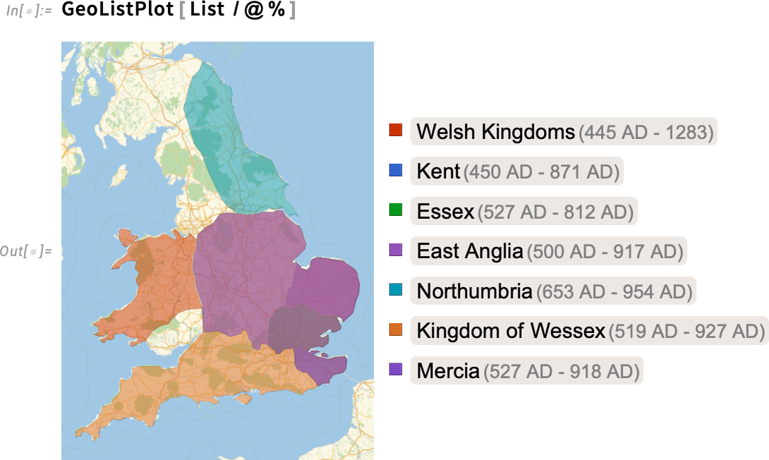
This then makes a map (the extra list makes these countries be rendered separately):
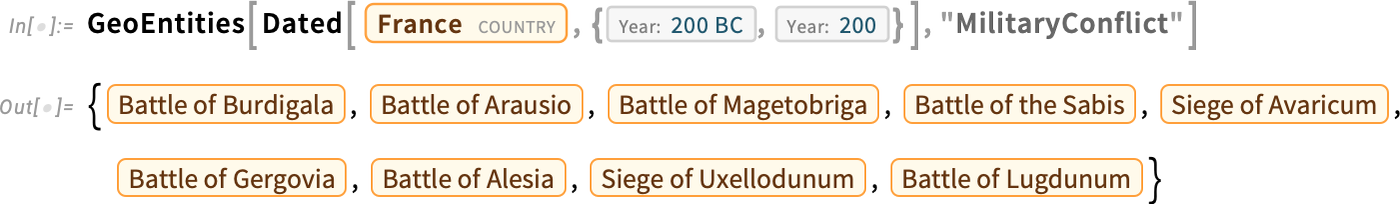
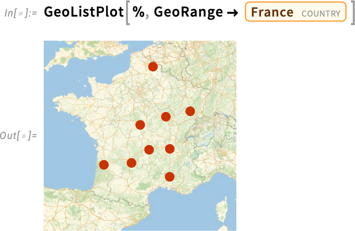
In the Wolfram Language we have data on quite a few kinds of historical entities beyond countries. For example, we have extensive data on military conflicts. Here we’re asking what military conflicts occurred within the borders of what’s now France between 200 BC and 200 AD:
Here’s a map of their locations:
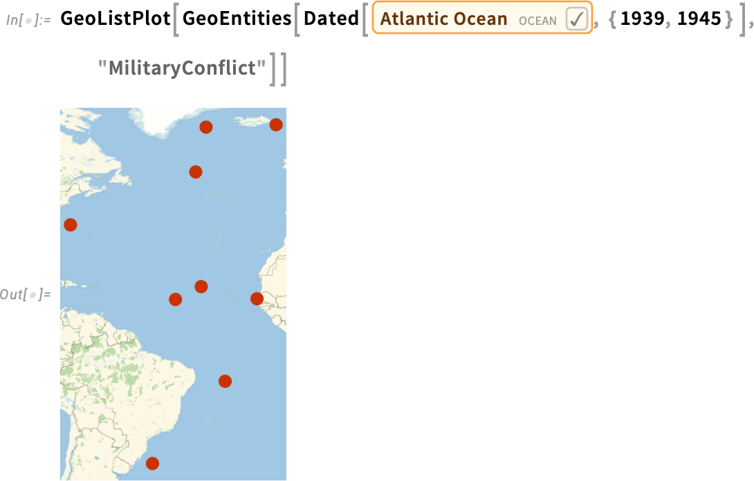
And here are conflicts in the Atlantic Ocean in the period 1939–1945:
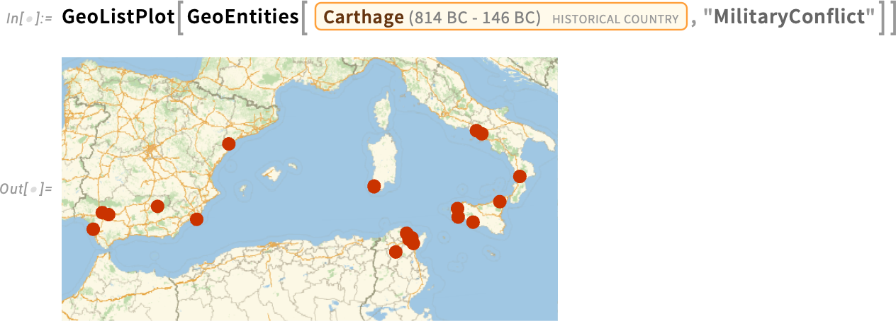
And—combining several things—here’s a map of conflicts that, at the time when they occurred, were within the region of what was then Carthage:
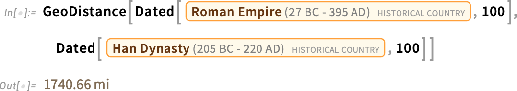
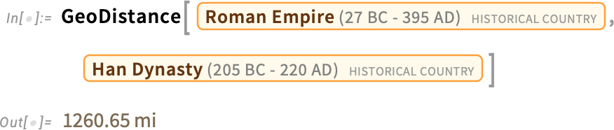
There are all sorts of things that we can compute from historical geography. For example, this asks for the (minimum) geo distance between the territory of the Roman Empire and the Han Dynasty in 100 AD:
But what about the overall minimum distance across all years when these historical countries existed? This gives the result for that:
Let’s compare this with a plot of these two entities:
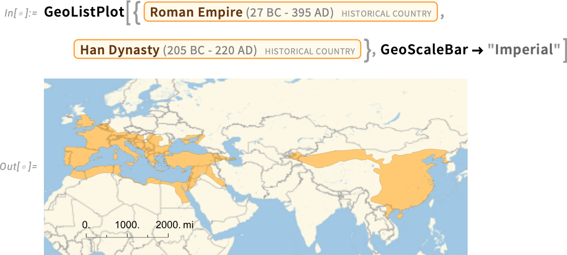
But there’s a subtlety here. What version of the Roman Empire is it that we’re showing on the map here? Our convention is by default to show historical countries “at their zenith”, i.e. at the moment when they had their maximum extent.
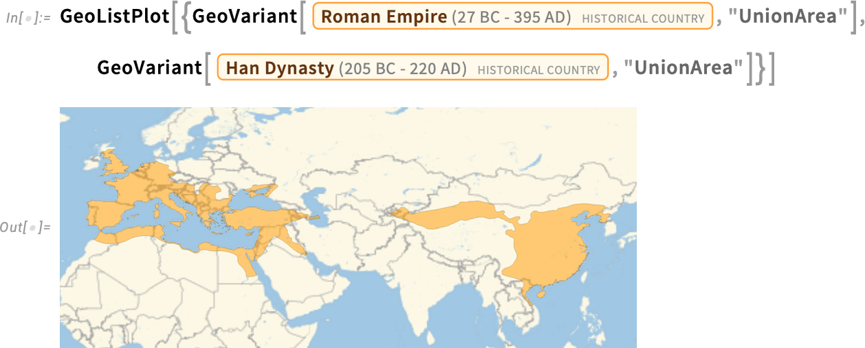
But what about other choices? Dated gives us a way to specify a particular date. But another possibility is to include in what we consider to be a particular historical country any territory that was ever part of that country, at any time in its history. And you can do this using GeoVariant[…, "UnionArea"]. In the particular case we’re showing here, it doesn’t make much difference, except that there’s more territory in Germany and Scotland included in the Roman Empire:
By the way, you can combine Dated and GeoVariant, to get things like “the zenith within a certain period” or “any territory that was included at any time within a period”. And, yes, it can get quite complicated. In a rather physics-like way you can think of the extent of a historical country as defining a region in spacetime—and indeed GeoVariant[…, "TimeSeries"] in effect represents a whole “stack of spacelike slices” in this spacetime region:
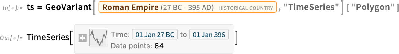
And—though it takes a little while—you can use it to make a video of the rise and fall of the Roman Empire:
Astronomical Graphics and Their Axes
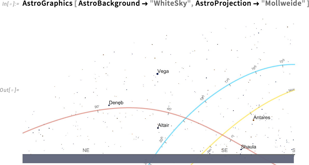
It’s complicated to define where things are in the sky. There are four main coordinate systems that get used in doing this: horizon (relative to local horizon), equatorial (relative to the Earth’s equator), ecliptic (relative to the orbit of the Earth around the Sun) and galactic (relative to the plane of the galaxy). And when we draw a diagram of the sky (here on white for clarity) it’s typical to show the “axes” for all these coordinate systems:

But here’s a tricky thing: how should those axes be labeled? Each one is different: horizon is most naturally labeled by things like cardinal directions (N, E, S, W, etc.), equatorial by hours in the day (in sidereal time), ecliptic by months in the year, and galactic by angle from the center of the galaxy.
In ordinary plots axes are usually straight, and labeled uniformly (or perhaps, say, logarithmically). But in astronomy things are much more complicated: the axes are intrinsically circular, and then get rendered through whatever projection we’re using.
And we might have thought that such axes would require some kind of custom structure. But not in the Wolfram Language. Because in the Wolfram Language we try to make things general. And axes are no exception:
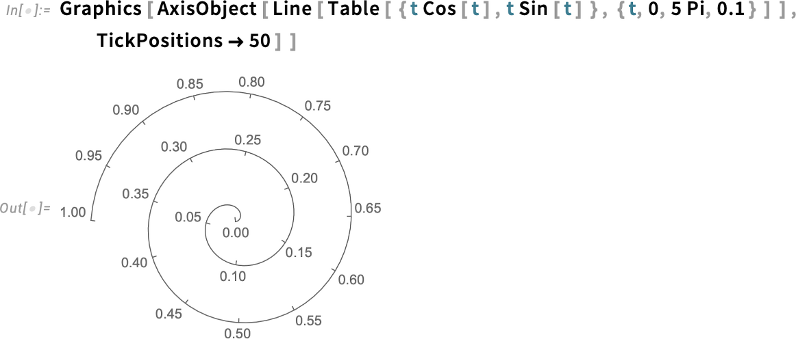
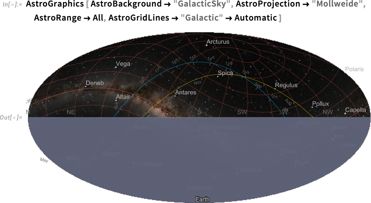
So in AstroGraphics all our various axes are just AxisObject constructs—that can be computed with. And so, for example, here’s a Mollweide projection of the sky:
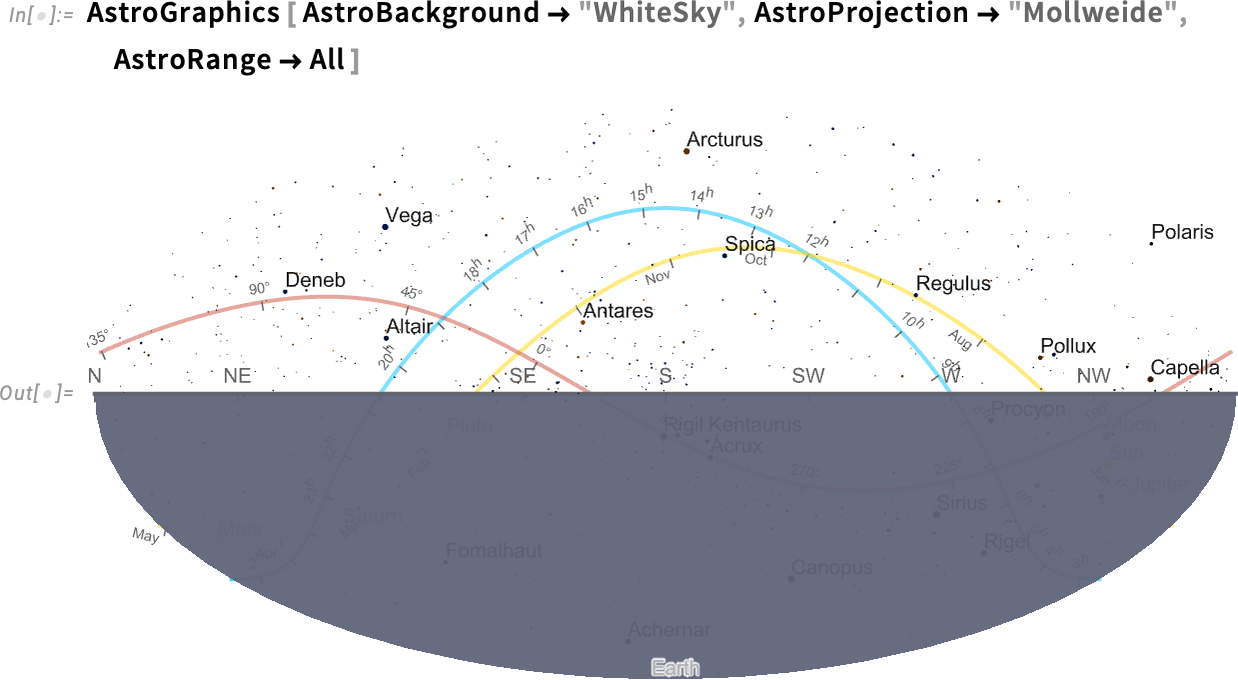
If we insist on “seeing the whole sky”, the bottom half is just the Earth (and, yes, the Sun isn’t shown because I’m writing this after it’s set for the day…):
Things get a bit wild if we start adding grid lines, here for galactic coordinates:
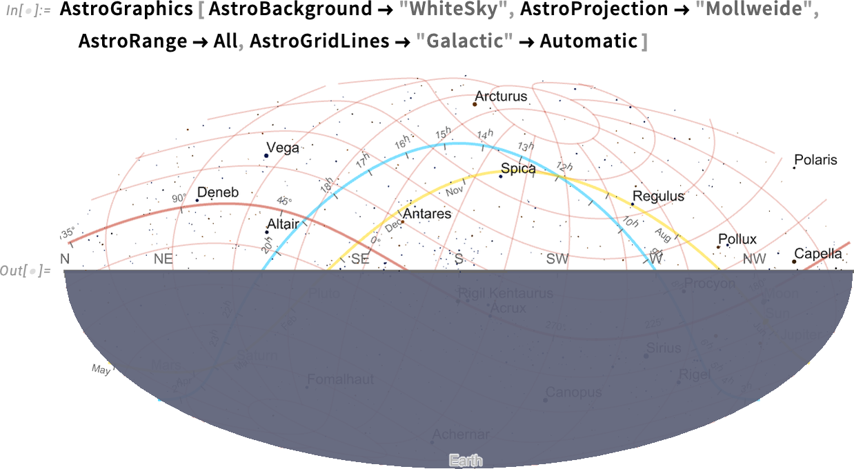
And, yes, the galactic coordinate axis is indeed aligned with the plane of the Milky Way (i.e. our galaxy):
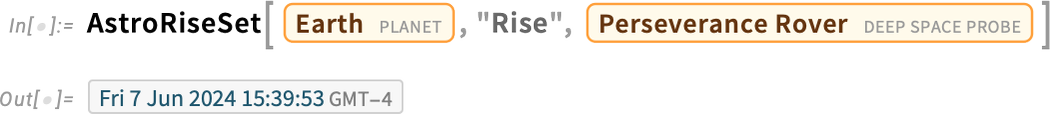
When Is Earthrise on Mars? New Level of Astronomical Computation
When will the Earth next rise above the horizon from where the Perseverance rover is on Mars? In Version 14.1 we can now compute this (and, yes, this is an “Earth time” converted from Mars time using the standard barycentric celestial reference system (BCRS) solar-system-wide spacetime coordinate system):
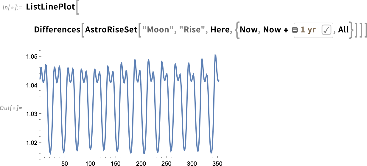
This is a fairly complicated computation that takes into account not only the motion and rotation of the bodies involved, but also various other physical effects. A more “down to Earth” example that one might readily check by looking out of one’s window is to compute the rise and set times of the Moon from a particular point on the Earth:
There’s a slight variation in the times between moonrises:

Over the course of a year we see systematic variations associated with the periods of different kinds of lunar months:
There are all sorts of subtleties here. For example, when exactly does one define something (like the Sun) to have “risen”? Is it when the top of the Sun first peeks out? When the center appears? Or when the “whole Sun” is visible? In Version 14.1 you can ask about any of these:
Oh, and you could compute the same thing for the rise of Venus, but now to see the differences, you’ve got to go to millisecond granularity (and, by the way, granularities of milliseconds down to picoseconds are new in Version 14.1):
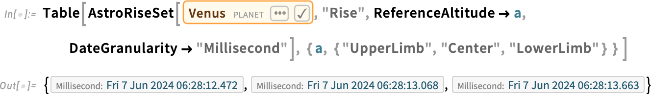
By the way, particularly for the Sun, the concept of ReferenceAltitude is useful in specifying the various kinds of sunrise and sunset: for example, “civil twilight” corresponds to a reference altitude of –6°.
Geometry Goes Color, and Polar
Last year we introduced the function ARPublish to provide a streamlined way to take 3D geometry and publish it for viewing in augmented reality. In Version 14.1 we’ve now extended this pipeline to deal with color:
(Yes, the color is a little different on the phone because the phone tries to make it look “more natural”.)

And now it’s easy to view this not just on a phone, but also, for example, on the Apple Vision Pro:
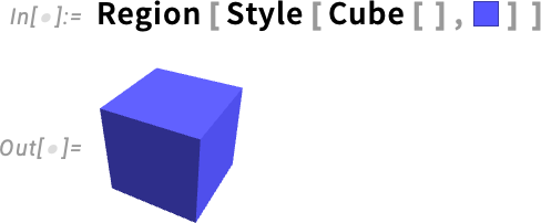
Graphics have always had color. But now in Version 14.1 symbolic geometric regions can have color too:
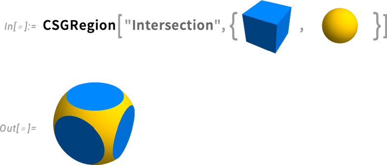
And constructive geometric operations on regions preserve color:
Two other new functions in Version 14.1 are PolarCurve and FilledPolarCurve:
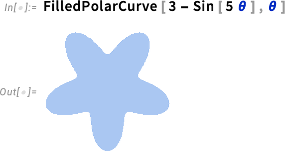
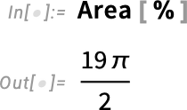
And while at this level this may look simple, what’s going on underneath is actually seriously complicated, with all sorts of symbolic analysis needed in order to determine what the “inside” of the parametric curve should be.
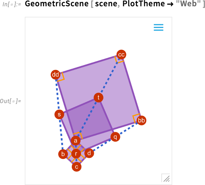
Talking about geometry and color brings up another enhancement in Version 14.1: plot themes for diagrams in synthetic geometry. Back in Version 12.0 we introduced symbolic synthetic geometry—in effect finally providing a streamlined computable way to do the kind of geometry that Euclid did two millennia ago. In the past few versions we’ve been steadily expanding our synthetic geometry capabilities, and now in Version 14.1 one notable thing we’ve added is the ability to use plot themes—and explicit graphics options—to style geometric diagrams. Here’s the default version of a geometric diagram:
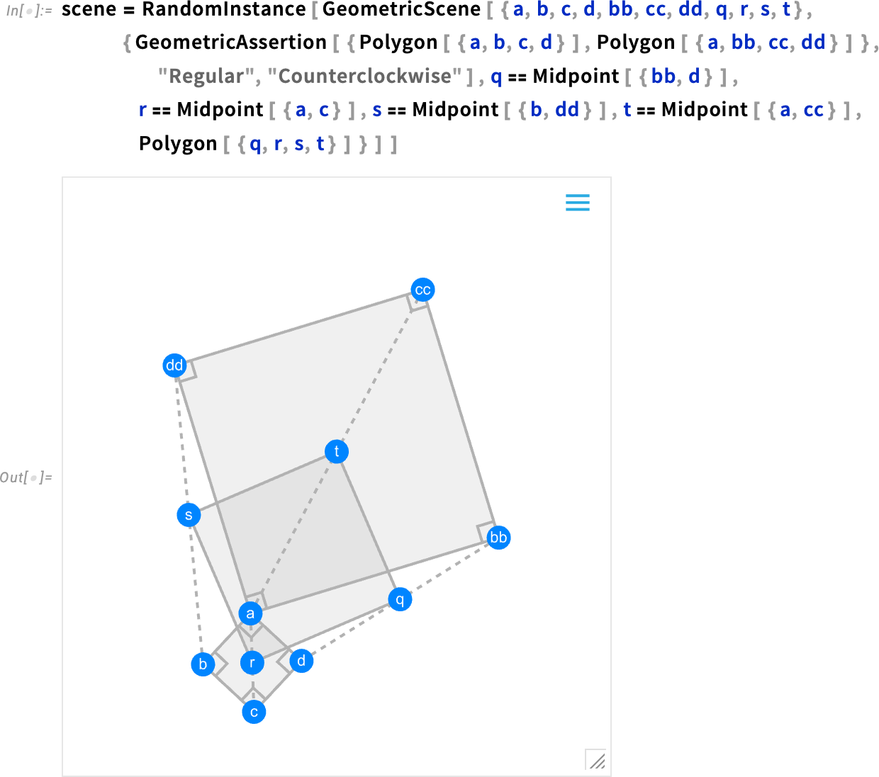
Now we can “theme” this for the web:
New Computation Flow in Notebooks: Introducing Cell-Linked %
In building up computations in notebooks, one very often finds oneself wanting to take a result one just got and then do something with it. And ever since Version 1.0 one’s been able to do this by referring to the result one just got as %. It’s very convenient. But there are some subtle and sometimes frustrating issues with it, the most important of which has to do with what happens when one reevaluates an input that contains %.
Let’s say you’ve done this:

But now you decide that actually you wanted Median[ % ^ 2 ] instead. So you edit that input and reevaluate it:

Oops! Even though what’s right above your input in the notebook is a list, the value of % is the latest result that was computed, which you can’t now see, but which was 3.
OK, so what can one do about this? We’ve thought about it for a long time (and by “long” I mean decades). And finally now in Version 14.1 we have a solution—that I think is very nice and very convenient. The core of it is a new notebook-oriented analog of %, that lets one refer not just to things like “the last result that was computed” but instead to things like “the result computed in a particular cell in the notebook”.
So let’s look at our sequence from above again. Let’s start typing another cell—say to “try to get it right”. In Version 14.1 as soon as we type % we see an autosuggest menu:

The menu is giving us a choice of (output) cells that we might want to refer to. Let’s pick the last one listed:

The ![]() object is a reference to the output from the cell that’s currently labeled In[1]—and using
object is a reference to the output from the cell that’s currently labeled In[1]—and using ![]() now gives us what we wanted.
now gives us what we wanted.
But let’s say we go back and change the first (input) cell in the notebook—and reevaluate it:

The cell now gets labeled In[5]—and the ![]() (in In[4]) that refers to that cell will immediately change to
(in In[4]) that refers to that cell will immediately change to ![]() :
:

And if we now evaluate this cell, it’ll pick up the value of the output associated with In[5], and give us a new answer:

So what’s really going on here? The key idea is that ![]() signifies a new type of notebook element that’s a kind of cell-linked analog of %. It represents the latest result from evaluating a particular cell, wherever the cell may be, and whatever the cell may be labeled. (The
signifies a new type of notebook element that’s a kind of cell-linked analog of %. It represents the latest result from evaluating a particular cell, wherever the cell may be, and whatever the cell may be labeled. (The ![]() object always shows the current label of the cell it’s linked to.) In effect
object always shows the current label of the cell it’s linked to.) In effect ![]() is “notebook front end oriented”, while ordinary % is kernel oriented.
is “notebook front end oriented”, while ordinary % is kernel oriented. ![]() is linked to the contents of a particular cell in a notebook; % refers to the state of the Wolfram Language kernel at a certain time.
is linked to the contents of a particular cell in a notebook; % refers to the state of the Wolfram Language kernel at a certain time.
![]() gets updated whenever the cell it’s referring to is reevaluated. So its value can change either through the cell being explicitly edited (as in the example above) or because reevaluation gives a different value, say because it involves generating a random number:
gets updated whenever the cell it’s referring to is reevaluated. So its value can change either through the cell being explicitly edited (as in the example above) or because reevaluation gives a different value, say because it involves generating a random number:

OK, so ![]() always refers to “a particular cell”. But what makes a cell a particular cell? It’s defined by a unique ID that’s assigned to every cell. When a new cell is created it’s given a universally unique ID, and it carries that same ID wherever it’s placed and whatever its contents may be (and even across different sessions). If the cell is copied, then the copy gets a new ID. And although you won’t explicitly see cell IDs,
always refers to “a particular cell”. But what makes a cell a particular cell? It’s defined by a unique ID that’s assigned to every cell. When a new cell is created it’s given a universally unique ID, and it carries that same ID wherever it’s placed and whatever its contents may be (and even across different sessions). If the cell is copied, then the copy gets a new ID. And although you won’t explicitly see cell IDs, ![]() works by linking to a cell with a particular ID.
works by linking to a cell with a particular ID.
One can think of ![]() as providing a “more stable” way to refer to outputs in a notebook. And actually, that’s true not just within a single session, but also across sessions. Say one saves the notebook above and opens it in a new session. Here’s what you’ll see:
as providing a “more stable” way to refer to outputs in a notebook. And actually, that’s true not just within a single session, but also across sessions. Say one saves the notebook above and opens it in a new session. Here’s what you’ll see:

The ![]() is now grayed out. So what happens if we try to reevaluate it? Well, we get this:
is now grayed out. So what happens if we try to reevaluate it? Well, we get this:

If we press Reconstruct from output cell the system will take the contents of the first output cell that was saved in the notebook, and use this to get input for the cell we’re evaluating:

In almost all cases the contents of the output cell will be sufficient to allow the expression “behind it” to be reconstructed. But in some cases—like when the original output was too big, and so was elided—there won’t be enough in the output cell to do the reconstruction. And in such cases it’s time to take the Go to input cell branch, which in this case will just take us back to the first cell in the notebook, and let us reevaluate it to recompute the output expression it gives.
By the way, whenever you see a “positional %” you can hover over it to highlight the cell it’s referring to:

Having talked a bit about “cell-linked %” it’s worth pointing out that there are still cases when you’ll want to use “ordinary %”. A typical example is if you have an input line that you’re using a bit like a function (say for post-processing) and that you want to repeatedly reevaluate to see what it produces when applied to your latest output.
In a sense, ordinary % is the “most volatile” in what it refers to. Cell-linked % is “less volatile”. But sometimes you want no volatility at all in what you’re referring to; you basically just want to burn a particular expression into your notebook. And in fact the % autosuggest menu gives you a way to do just that.
Notice the ![]() that appears in whatever row of the menu you’re selecting:
that appears in whatever row of the menu you’re selecting:

Press this and you’ll insert (in iconized form) the whole expression that’s being referred to:

Now—for better or worse—whatever changes you make in the notebook won’t affect the expression, because it’s right there, in literal form, “inside” the icon. And yes, you can explicitly “uniconize” to get back the original expression:

Once you have a cell-linked % it always has a contextual menu with various actions:

One of those actions is to do what we just mentioned, and replace the positional ![]() by an iconized version of the expression it’s currently referring to. You can also highlight the output and input cells that the
by an iconized version of the expression it’s currently referring to. You can also highlight the output and input cells that the ![]() is “linked to”. (Incidentally, another way to replace a
is “linked to”. (Incidentally, another way to replace a ![]() by the expression it’s referring to is simply to “evaluate in place”
by the expression it’s referring to is simply to “evaluate in place” ![]() , which you can do by selecting it and pressing CMDReturn or ShiftControlEnter.)
, which you can do by selecting it and pressing CMDReturn or ShiftControlEnter.)
Another item in the ![]() menu is Replace With Rolled-Up Inputs. What this does is—as it says—to “roll up” a sequence of “
menu is Replace With Rolled-Up Inputs. What this does is—as it says—to “roll up” a sequence of “![]() references” and create a single expression from them:
references” and create a single expression from them:

What we’ve talked about so far one can think of as being “normal and customary” uses of ![]() . But there are all sorts of corner cases that can show up. For example, what happens if you have a
. But there are all sorts of corner cases that can show up. For example, what happens if you have a ![]() that refers to a cell you delete? Well, within a single (kernel) session that’s OK, because the expression “behind” the cell is still available in the kernel (unless you reset your $HistoryLength etc.). Still, the
that refers to a cell you delete? Well, within a single (kernel) session that’s OK, because the expression “behind” the cell is still available in the kernel (unless you reset your $HistoryLength etc.). Still, the ![]() will show up with a “red broken link” to indicate that “there could be trouble”:
will show up with a “red broken link” to indicate that “there could be trouble”:
![]()
And indeed if you go to a different (kernel) session there will be trouble—because the information you need to get the expression to which the ![]() refers is simply no longer available, so it has no choice but to show up in a kind of everything-has-fallen-apart “surrender state” as:
refers is simply no longer available, so it has no choice but to show up in a kind of everything-has-fallen-apart “surrender state” as:
![]()
![]() is primarily useful when it refers to cells in the notebook you’re currently using (and indeed the autosuggest menu will contain only cells from your current notebook). But what if it ends up referring to a cell in a different notebook, say because you copied the cell from one notebook to another? It’s a precarious situation. But if all relevant notebooks are open,
is primarily useful when it refers to cells in the notebook you’re currently using (and indeed the autosuggest menu will contain only cells from your current notebook). But what if it ends up referring to a cell in a different notebook, say because you copied the cell from one notebook to another? It’s a precarious situation. But if all relevant notebooks are open, ![]() can still work, though it’s displayed in purple with an action-at-a-distance “wi-fi icon” to indicate its precariousness:
can still work, though it’s displayed in purple with an action-at-a-distance “wi-fi icon” to indicate its precariousness:
![]()
And if, for example, you start a new session, and the notebook containing the “source” of the ![]() isn’t open, then you’ll get the “surrender state”. (If you open the necessary notebook it’ll “unsurrender” again.)
isn’t open, then you’ll get the “surrender state”. (If you open the necessary notebook it’ll “unsurrender” again.)
Yes, there are lots of tricky cases to cover (in fact, many more than we’ve explicitly discussed here). And indeed seeing all these cases makes us not feel bad about how long it’s taken for us to conceptualize and implement ![]() .
.
The most common way to access ![]() is to use the % autosuggest menu. But if you know you want a
is to use the % autosuggest menu. But if you know you want a ![]() , you can always get it by “pure typing”, using for example ESC%ESC. (And, yes, ESC%%ESC or ESC%5ESC etc. also work, so long as the necessary cells are present in your notebook.)
, you can always get it by “pure typing”, using for example ESC%ESC. (And, yes, ESC%%ESC or ESC%5ESC etc. also work, so long as the necessary cells are present in your notebook.)
The UX Journey Continues: New Typing Affordances, and More
We invented Wolfram Notebooks more than 36 years ago, and we’ve been improving and polishing them ever since. And in Version 14.1 we’re implementing several new ideas, particularly around making it even easier to type Wolfram Language code.
It’s worth saying at the outset that good UX ideas quickly become essentially invisible. They just give you hints about how to interpret something or what to do with it. And if they’re doing their job well, you’ll barely notice them, and everything will just seem “obvious”.
So what’s new in UX for Version 14.1? First, there’s a story around brackets. We first introduced syntax coloring for unmatched brackets back in the late 1990s, and gradually polished it over the following two decades. Then in 2021 we started “automatching” brackets (and other delimiters), so that as soon as you type “f[” you immediately get f[ ].
But how do you keep on typing? You could use an ![]() to “move through” the ]. But we’ve set it up so you can just “type through” ] by typing ]. In one of those typical pieces of UX subtlety, however, “type through” doesn’t always make sense. For example, let’s say you typed f[x]. Now you click right after [ and you type g[, so you’ve got f[g[x]. You might think there should be an autotyped ] to go along with the [ after g. But where should it go? Maybe you want to get f[g[x]], or maybe you’re really trying to type f[g[],x]. We definitely don’t want to autotype ] in the wrong place. So the best we can do is not autotype anything at all, and just let you type the ] yourself, where you want it. But remember that with f[x] on its own, the ] is autotyped, and so if you type ] yourself in this case, it’ll just type through the autotyped ] and you won’t explicitly see it.
to “move through” the ]. But we’ve set it up so you can just “type through” ] by typing ]. In one of those typical pieces of UX subtlety, however, “type through” doesn’t always make sense. For example, let’s say you typed f[x]. Now you click right after [ and you type g[, so you’ve got f[g[x]. You might think there should be an autotyped ] to go along with the [ after g. But where should it go? Maybe you want to get f[g[x]], or maybe you’re really trying to type f[g[],x]. We definitely don’t want to autotype ] in the wrong place. So the best we can do is not autotype anything at all, and just let you type the ] yourself, where you want it. But remember that with f[x] on its own, the ] is autotyped, and so if you type ] yourself in this case, it’ll just type through the autotyped ] and you won’t explicitly see it.
So how can you tell whether a ] you type will explicitly show up, or will just be “absorbed” as type-through? In Version 14.1 there’s now different syntax coloring for these cases: yellow if it’ll be “absorbed”, and pink if it’ll explicitly show up.
This is an example of non-type-through, so Range is colored yellow and the ] you type is “absorbed”:
![]()
And this is an example of non-type-through, so Round is colored pink and the ] you type is explicitly inserted:
![]()
This may all sound very fiddly and detailed—and for us in developing it, it is. But the point is that you don’t explicitly have to think about it. You quickly learn to just “take the hint” from the syntax coloring about when your closing delimiters will be “absorbed” and when they won’t. And the result is that you’ll have an even smoother and faster typing experience, with even less chance of unmatched (or incorrectly matched) delimiters.
The new syntax coloring we just discussed helps in typing code. In Version 14.1 there’s also something new that helps in reading code. It’s an enhanced version of something that’s actually common in IDEs: when you click (or select) a variable, every instance of that variable immediately gets highlighted:

What’s subtle in our case is that we take account of the scoping of localized variables—putting a more colorful highlight on instances of a variable that are in scope:

One place this tends to be particularly useful is in understanding nested pure functions that use #. By clicking a # you can see which other instances of # are in the same pure function, and which are in different ones (the highlight is bluer inside the same function, and grayer outside):
![]()
On the subject of finding variables, another change in Version 14.1 is that fuzzy name autocompletion now also works for contexts. So if you have a symbol whose full name is context1`subx`var2 you can type c1x and you’ll get a completion for the context; then accept this and you get a completion for the symbol.
There are also several other notable UX “tune-ups” in Version 14.1. For many years, there’s been an “information box” that comes up whenever you hover over a symbol. Now that’s been extended to entities—so (alongside their explicit form) you can immediately get to information about them and their properties:
![]()
Next there’s something that, yes, I personally have found frustrating in the past. Say you’ve a file, or an image, or something else somewhere on your computer’s desktop. Normally if you want it in a Wolfram Notebook you can just drag it there, and it will very beautifully appear. But what if the thing you’re dragging is very big, or has some other kind of issue? In the past, the drag just failed. Now what happens is that you get the explicit Import that the dragging would have done, so that you can run it yourself (getting progress information, etc.), or you can modify it, say adding relevant options.
Another small piece of polish that’s been added in Version 14.1 has to do with Preferences. There are a lot of things you can set in the notebook front end. And they’re explained, at least briefly, in the many Preferences panels. But in Version 14.1 there are now (i) buttons that give direct links to the relevant workflow documentation:

Syntax for Natural Language Input
Ever since shortly after Wolfram|Alpha was released in 2009, there’ve been ways to access its natural language understanding capabilities in the Wolfram Language. Foremost among these has been CTRL=—which lets you type free-form natural language and immediately get a Wolfram Language version, often in terms of entities, etc.:
![]()
Generally this is a very convenient and elegant capability. But sometimes one may want to just use plain text to specify natural language input, for example so that one doesn’t interrupt one’s textual typing of input.
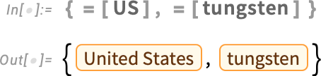
In Version 14.1 there’s a new mechanism for this: syntax for directly entering free-form natural language input. The syntax is a kind of a “textified” version of CTRL=: =[…]. When you type =[...] as input nothing immediately happens. It’s only when you evaluate your input that the natural language gets interpreted—and then whatever it specifies is computed.
Here’s a very simple example, where each =[…] just turns into an entity:
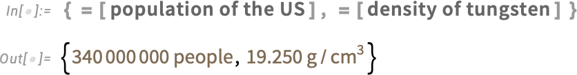
But when the result of interpreting the natural language is an expression that can be further evaluated, what will come out is the result of that evaluation:
One feature of using =[…] instead of CTRL= is that =[…] is something anyone can immediately see how to type:
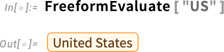
But what actually is =[…]? Well, it’s just input syntax for the new function FreeformEvaluate:
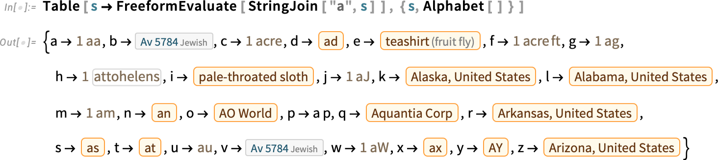
You can use FreeformEvaluate inside a program—here, rather whimsically, to see what interpretations are chosen by default for “a” followed by each letter of the alphabet:
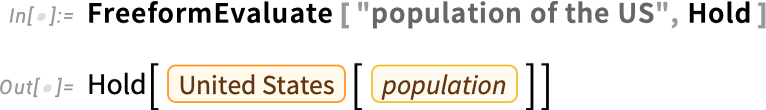
By default, FreeformEvaluate interprets your input, then evaluates it. But you can also specify that you want to hold the result of the interpretation:
Diff[ ] … for Notebooks and More!
It’s been a very long-requested capability: give me a way to tell what changed, particularly in a notebook. It’s fairly easy to do “diffs” for plain text. But for notebooks—as structured symbolic documents—it’s a much more complicated story. But in Version 14.1 it’s here! We’ve got a function Diff for doing diffs in notebooks, and actually also in many other kinds of things.
Here’s an example, where we’re requesting a “side-by-side view” of the diff between two notebooks:
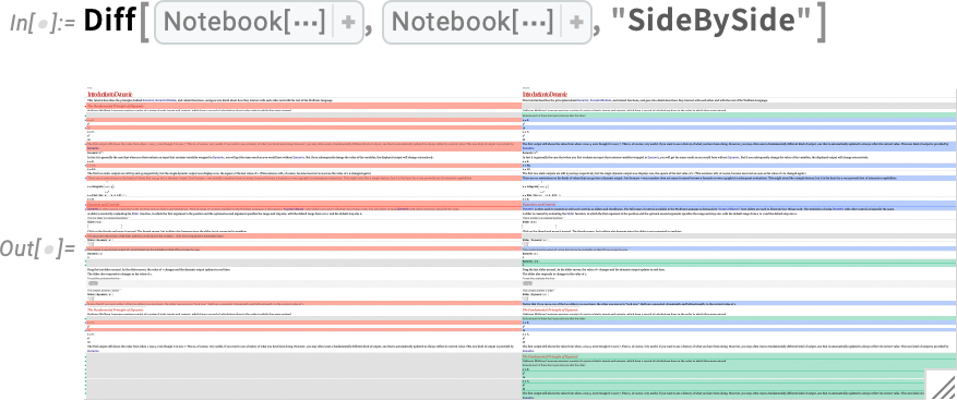
And here’s an “alignment chart view” of the diff:

Like everything else in the Wolfram Language, a “diff” is a symbolic expression. Here’s an example:
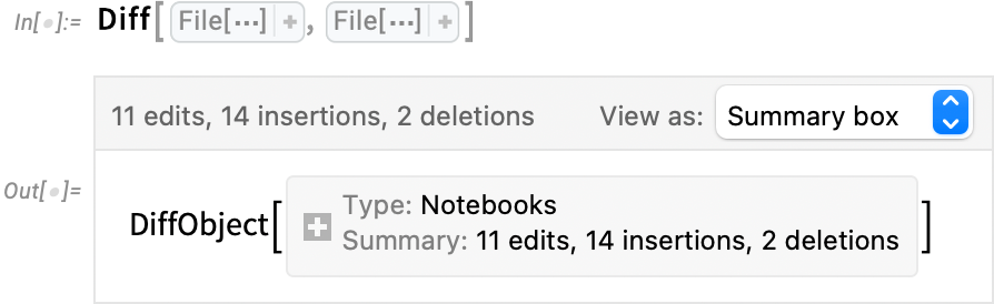
There are lots of different ways to display a diff object; many of them one can select interactively with the menu:

But the most important thing about diff objects is that they can be used programmatically. And in particular DiffApply applies the diffs from a diff object to an existing object, say a notebook.
What’s the point of this? Well, let’s imagine you’ve made a notebook, and given a copy of it to someone else. Then both you and the person to whom you’ve given the copy make changes. You can create a diff object of the diffs between the original version of the notebook, and the version with your changes. And if the changes the other person made don’t overlap with yours, you can just take your diffs and use DiffApply to apply your diffs to their version, thereby getting a “merged notebook” with both sets of changes made.
But what if your changes might conflict? Well, then you need to use the function Diff3. Diff3 takes your original notebook and two modified versions, and does a “three-way diff” to give you a diff object in which any conflicts are explicitly identified. (And, yes, three-way diffs are familiar from source control systems in which they provide the back end for making the merging of files as automated as possible.)
Notebooks are an important use case for Diff and related functions. But they’re not the only one. Diff can perfectly well be applied, for example, just to lists:
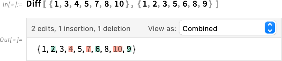
There are many ways to display this diff object; here’s a side-by-side view:

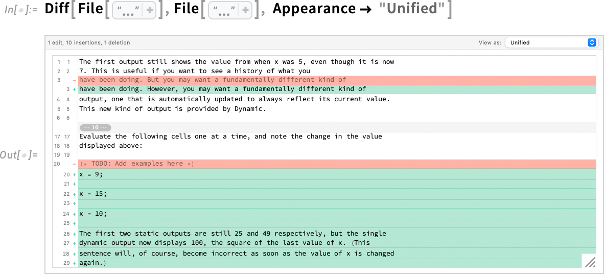
And here’s a “unified view” reminiscent of how one might display diffs for lines of text in a file:

And, speaking of files, Diff, etc. can immediately be applied to files:
Diff, etc. can also be applied to cells, where they can analyze changes in both content and styles or metadata. Here we’re creating two cells and then diffing them—showing the result in a side by side:
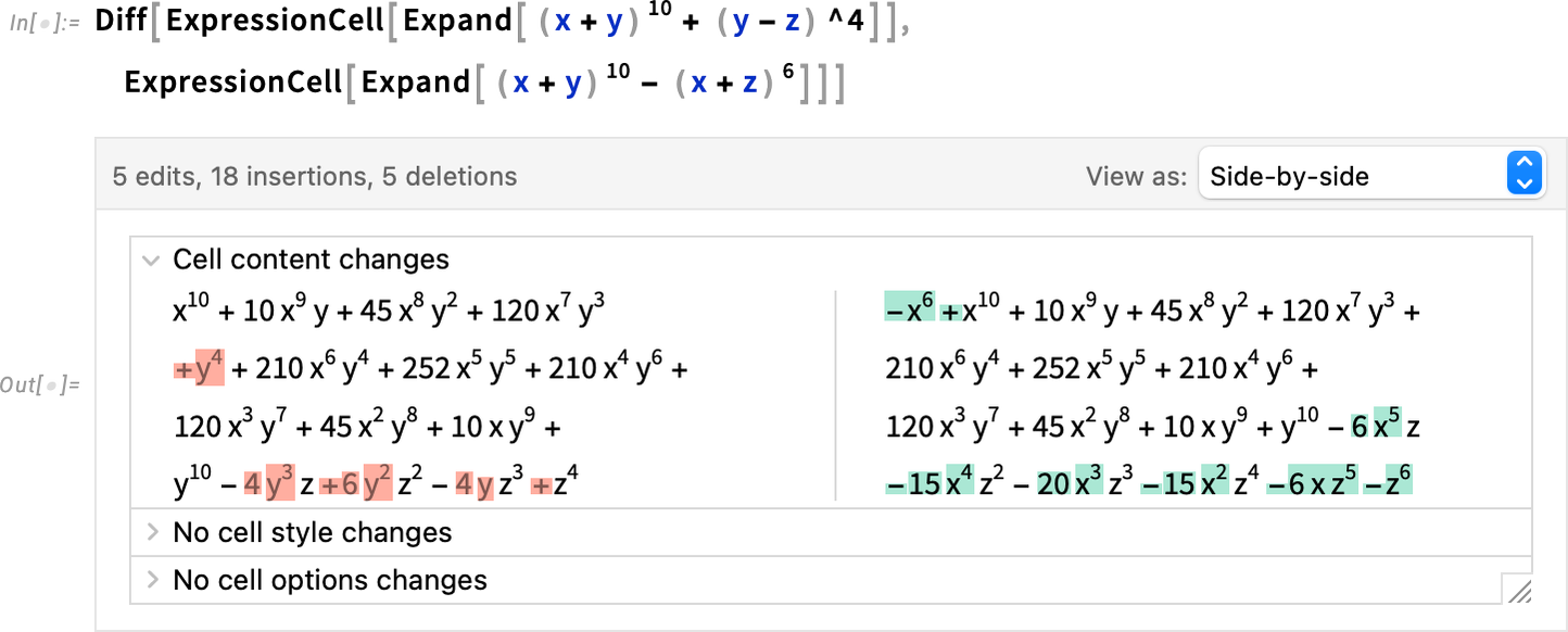
In “Combined” view the “pure insertions” are highlighted in green, the “pure deletions” in red, and the “edits” are shown as deletion/insertion stacks:

Many uses of diff technology revolve around content development—editing, software engineering, etc. But in the Wolfram Language Diff, etc. are set up also to be convenient for information visualization and for various kinds of algorithmic operations. For example, to see what letters differ between the Spanish and Polish alphabets, we can just use Diff:
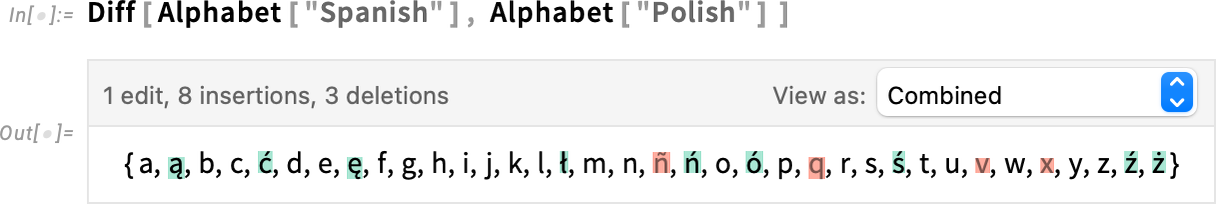
Here’s the “pure visualization”:
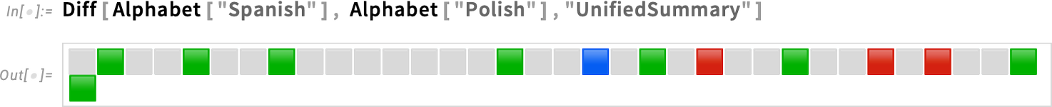
And here’s an alternate “unified summary” form:
Another use case for Diff is bioinformatics. We retrieve two genome sequences—as strings—then use Diff:
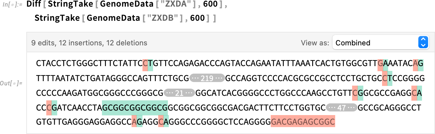
We can take the resulting diff object and show it in a different form—here character alignment:
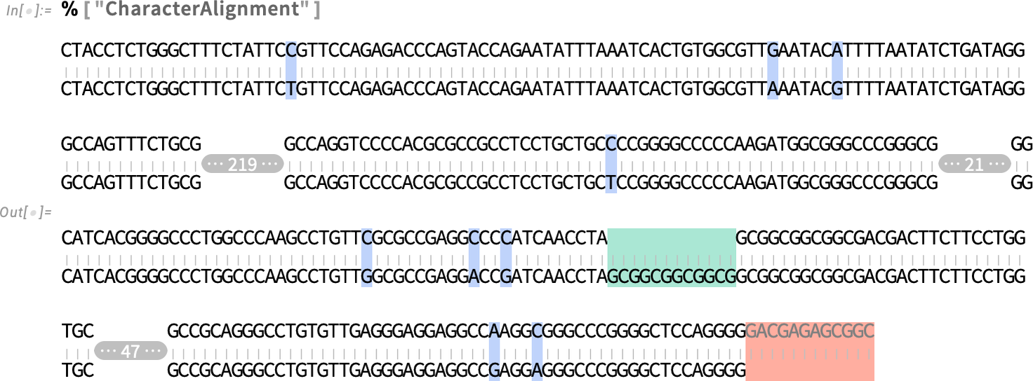
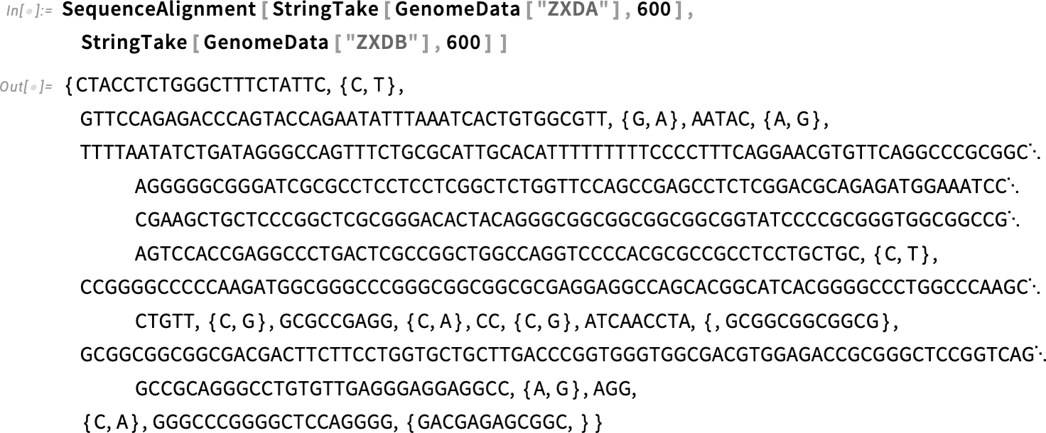
Under the hood, by the way, Diff is finding the differences using SequenceAlignment. But while Diff is giving a “high-level symbolic diff object”, SequenceAlignment is giving a direct low-level representation of the sequence alignment:
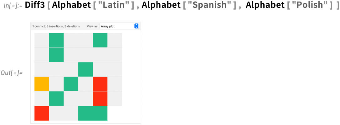
Information visualization isn’t restricted to two-way diffs; here’s an example with a three-way diff:
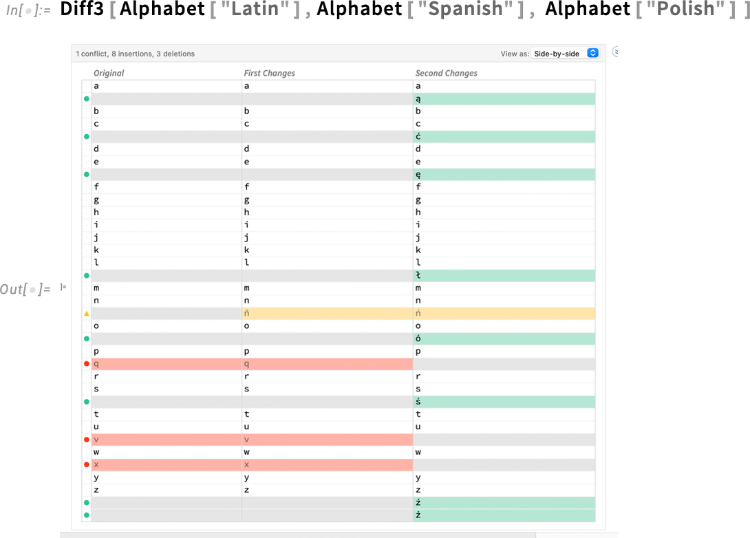
And here it is as a “unified summary”:
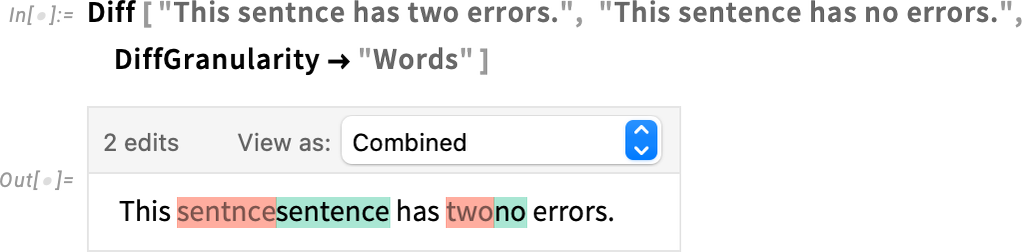
There are all sorts of options for diffs. One that is sometimes important is DiffGranularity. By default the granularity for diffs of strings is "Characters":
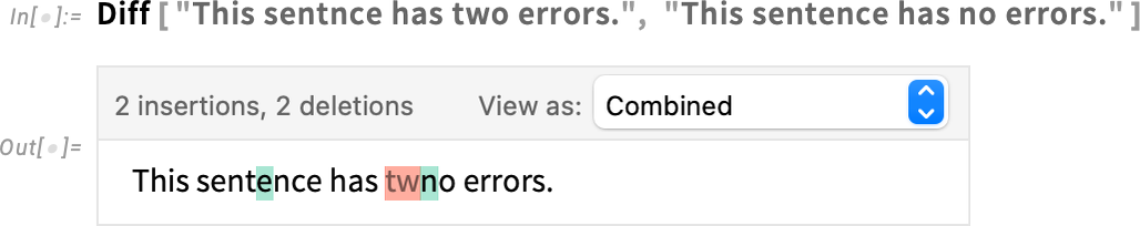
But it’s also possible to set it to be "Words":
Coming back to notebooks, the most “interactive” form of diff is a “report”:
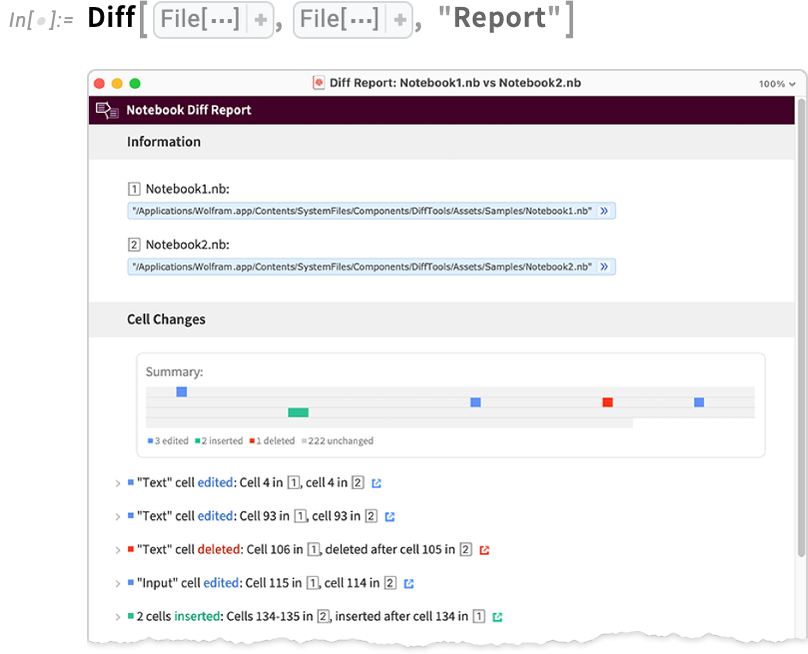
In such a report, you can open cells to see the details of a specific change, and you can also click to jump to where the change occurred in the underlying notebooks.
When it comes to analyzing notebooks, there’s another new feature in Version 14.1: NotebookCellData. NotebookCellData gives you direct programmatic access to lots of properties of notebooks. By default it generates a dataset of some of them, here for the notebook in which I’m currently authoring this:
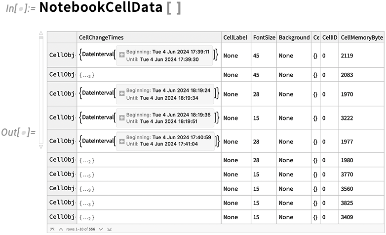
There are properties like the word count in each cell, the style of each cell, the memory footprint of each cell, and a thumbnail image of each cell.
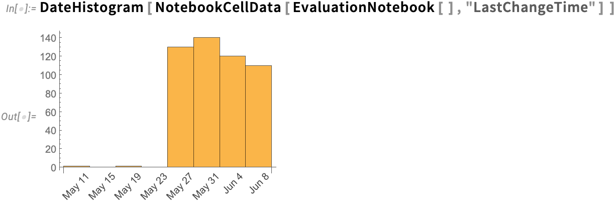
Ever since Version 6 in 2007 we’ve had the CellChangeTimes option which records when cells in notebooks are created or modified. And now in Version 14.1 NotebookCellData provides direct programmatic access to this data. So, for example, here’s a date histogram of when the cells in the current notebook were last changed:
Lots of Little Language Tune-Ups
It’s part of a journey of almost four decades. Steadily discovering—and inventing—new “lumps of computational work” that make sense to implement as functions or features in the Wolfram Language. The Wolfram Language is of course very much strong enough that one can build essentially any functionality from the primitives that already exist in it. But part of the point of the language is to define the best “elements of computational thought”. And particularly as the language progresses, there’s a continual stream of new opportunities for convenient elements that get exposed. And in Version 14.1 we’ve implemented quite a diverse collection of them.
Let’s say you want to nestedly compose a function. Ever since Version 1.0 there’s been Nest for that:
But what if you want the abstract nested function, not yet applied to anything? Well, in Version 14.1 there’s now an operator form of Nest (and NestList) that represents an abstract nested function that can, for example, be composed with other functions, as in
or equivalently:
A decade ago we introduced functions like AllTrue and AnyTrue that effectively “in one gulp” do a whole collection of separate tests. If one wanted to test whether there are any primes in a list, one can always do:
But it’s better to “package” this “lump of computational work” into the single function AnyTrue:
In Version 14.1 we’re extending this idea by introducing AllMatch, AnyMatch and NoneMatch:
Another somewhat related new function is AllSameBy. SameQ tests whether a collection of expressions are immediately the same. AllSameBy tests whether expressions are the same by the criterion that the value of some function applied to them is the same:
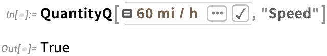
Talking of tests, another new feature in Version 14.1 is a second argument to QuantityQ (and KnownUnitQ), which lets you test not only whether something is a quantity, but also whether it’s a specific type of physical quantity:
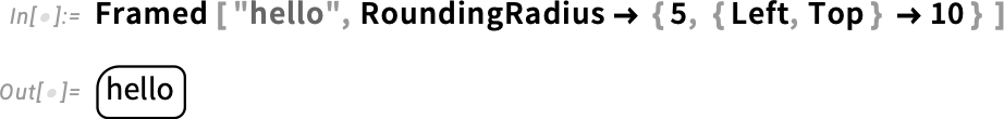
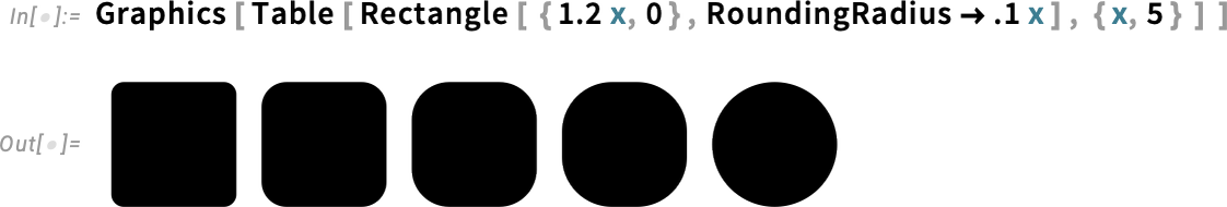
And now talking about “rounding things out”, Version 14.1 does that in a very literal way by enhancing the RoundingRadius option. For a start, you can now specify a different rounding radius for particular corners:
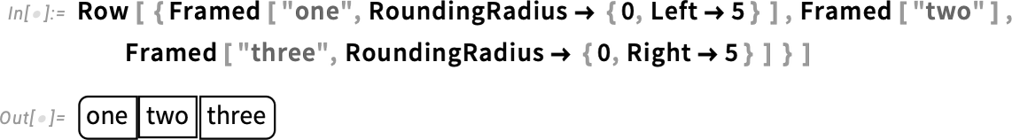
And, yes, that’s useful if you’re trying to fit button-like constructs together:
By the way, RoundingRadius now also works for rectangles inside Graphics:
Let’s say you have a string, like “hello”. There are many functions that operate directly on strings. But sometimes you really just want to use a function that operates on lists—and apply it to the characters in a string. Now in Version 14.1 you can do this using StringApply:
Another little convenience in Version 14.1 is the function BitFlip, which, yes, flips a bit in the binary representation of a number:
When it comes to Boolean functions, a detail that’s been improved in Version 14.1 is the conversion to NAND representation. By default, functions like BooleanConvert have allowed Nand[p] (which is equivalent to Not[p]). But in Version 14.1 there’s now "BinaryNAND" which yields for example Nand[p, p] instead of just Nand[p] (i.e. Not[p]). So here’s a representation of Or in terms of Nand:
Making the Wolfram Compiler Easier to Use
Let’s say you have a piece of Wolfram Language code that you know you’re going to run a zillion times—so you want it to run absolutely as fast as possible. Well, you’ll want to make sure you’re doing the best algorithmic things you can (and making the best possible use of Wolfram Language superfunctions, etc.). And perhaps you’ll find it helpful to use things like DataStructure constructs. But ultimately if you really want your code to run absolutely as fast as your computer can make it, you’ll probably want to set it up so that it can be compiled using the Wolfram Compiler, directly to LLVM code and then machine code.
We’ve been developing the Wolfram Compiler for many years, and it’s becoming steadily more capable (and efficient). And for example it’s become increasingly important in our own internal development efforts. In the past, when we wrote critical inner-loop internal code for the Wolfram Language, we did it in C. But in the past few years we’ve almost completely transitioned instead to writing pure Wolfram Language code that we then compile with the Wolfram Compiler. And the result of this has been a dramatically faster and more reliable development pipeline for writing inner-loop code.
Ultimately what the Wolfram Compiler needs to do is to take the code you write and align it with the low-level capabilities of your computer, figuring out what low-level data types can be used for what, etc. Some of this can be done automatically (using all sorts of fancy symbolic and theorem-proving-like techniques). But some needs to be based on collaboration between the programmer and the compiler. And in Version 14.1 we’re adding several important ways to enhance that collaboration.
The first thing is that it’s now easy to get access to information the compiler has. For example, here’s the type declaration the compiler has for the built-in function Dimensions:
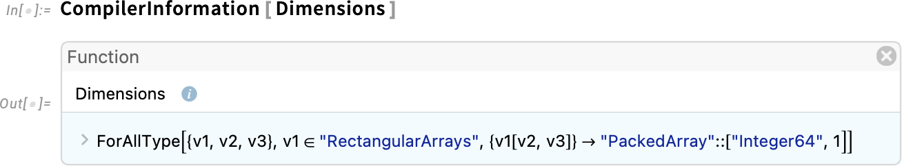
And here’s the source code of the actual implementation the compiler is using for Dimensions, calling its intrinsic low-level internal functions like CopyTo:

A function like Map has a vastly more complex set of type declarations:
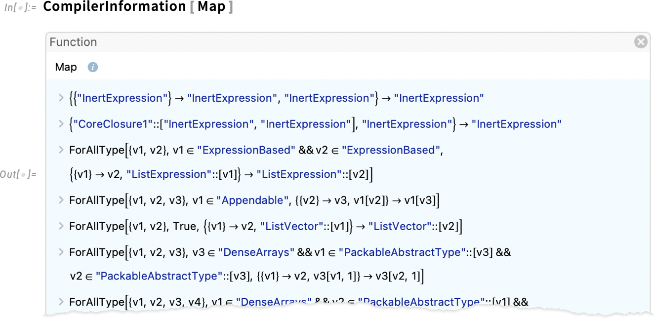
For types themselves, CompilerInformation lets you see their type hierarchy:
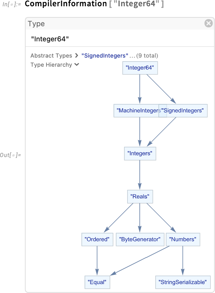
And for data structure types, you can do things like see the fields they contain, and the operations they support:
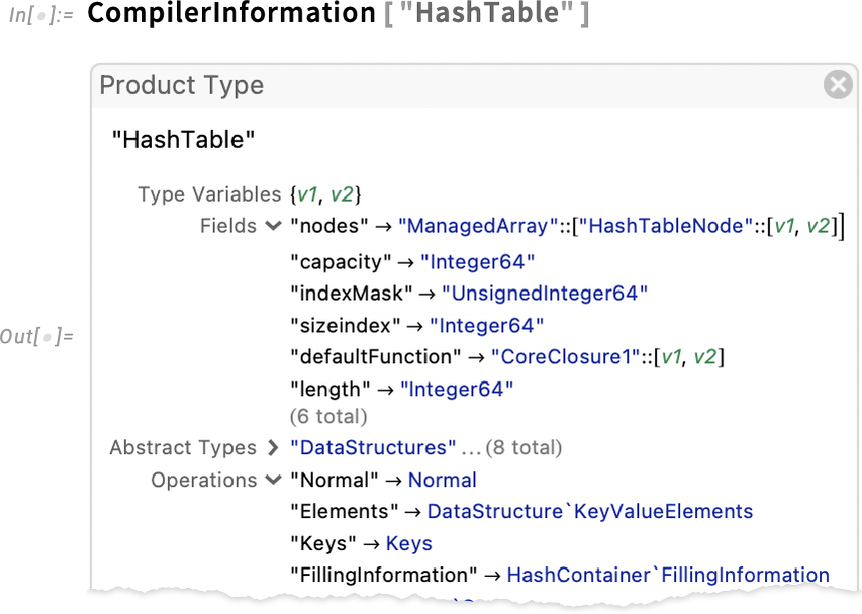
And, by the way, something new in Version 14.1 is the function OperationDeclaration which lets you declare operations to add to a data structure type you’ve defined.
Once you actually start running the compiler, a convenient new feature in Version 14.1 is a detailed progress monitor that lets you see what the compiler is doing at each step:
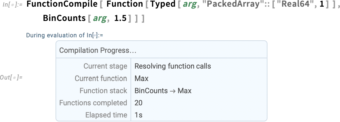
As we said, the key to compilation is figuring out how to align your code with the low-level capabilities of your computer. The Wolfram Language can do arbitrary symbolic operations. But many of those don’t align with low-level capabilities of your computer, and can’t meaningfully be compiled. Sometimes those failures to align are the result of sophistication that’s possible only with symbolic operations. But sometimes the failures can be avoided if you “unpack” things a bit. And sometimes the failures are just the result of programming mistakes. And now in Version 14.1 the Wolfram Compiler is starting to be able to annotate your code to show where the misalignments are happening, so you can go through and figure out what to do with them. (It’s something that’s uniquely possible because of the symbolic structure of the Wolfram Language and even more so of Wolfram Notebooks.)
Here’s a very simple example:

In compiled code, Sin expects a numerical argument, so a Boolean argument won’t work. Clicking the Source button lets you see where specifically something went wrong:

If you have several levels of definitions, the Source button will show you the whole chain:
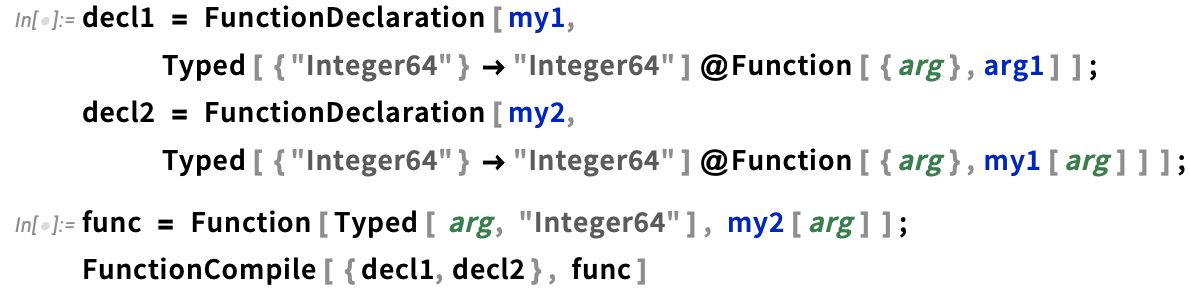
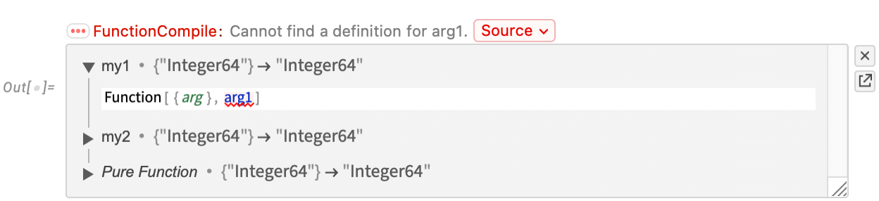
Here’s a slightly more complicated piece of code, in which the specific place where there’s a problem is highlighted:
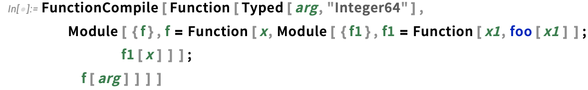
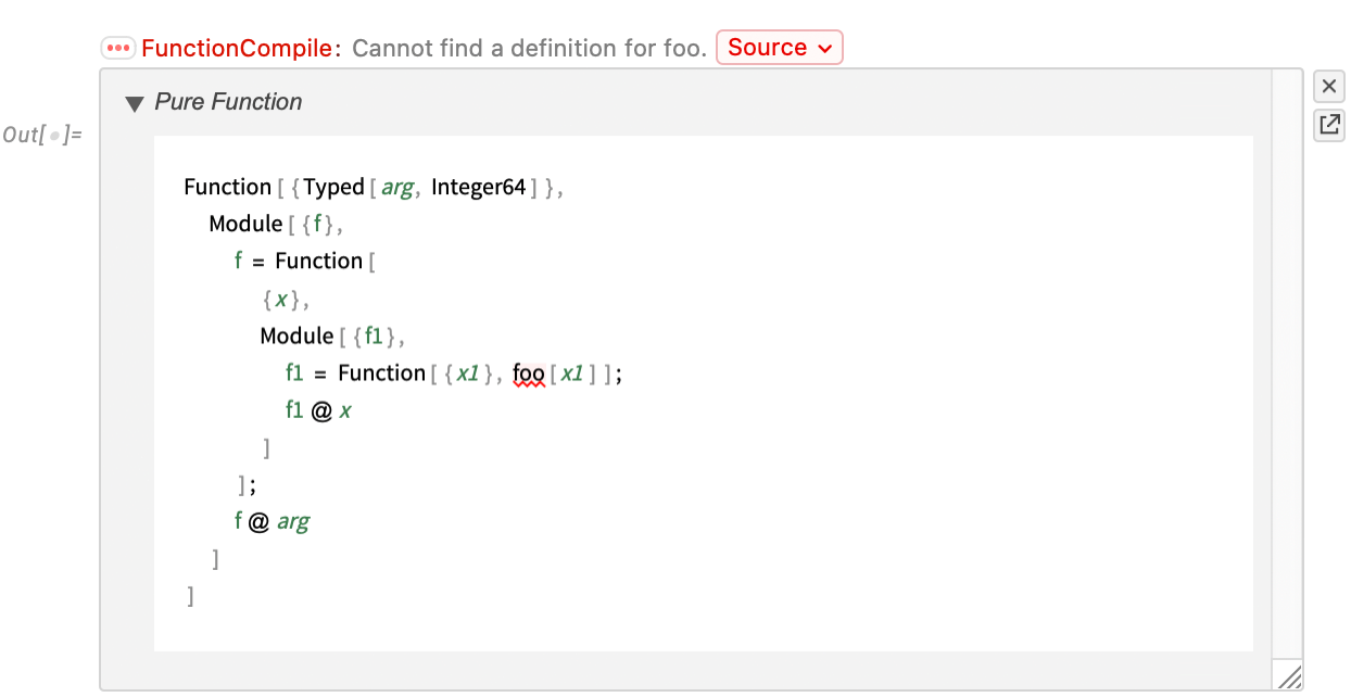
In a typical workflow you might start from pure Wolfram Language code, without Typed and other compilation information. Then you start adding such information, repeatedly trying the compilation, seeing what issues arise, and fixing them. And, by the way, because it’s completely efficient to call small pieces of compiled code within ordinary Wolfram Language code, it’s common to start by annotating and compiling the “innermost inner loops” in your code, and gradually “working outwards”.
But, OK, let’s say you’ve successfully compiled a piece of code. Most of the time it’ll handle certain cases, but not others (for example, it might work fine with machine-precision numbers, but not be capable of handling arbitrary precision). By default, compiled code that’s running is set up to generate a message and revert to ordinary Wolfram Language evaluation if it can’t handle something:
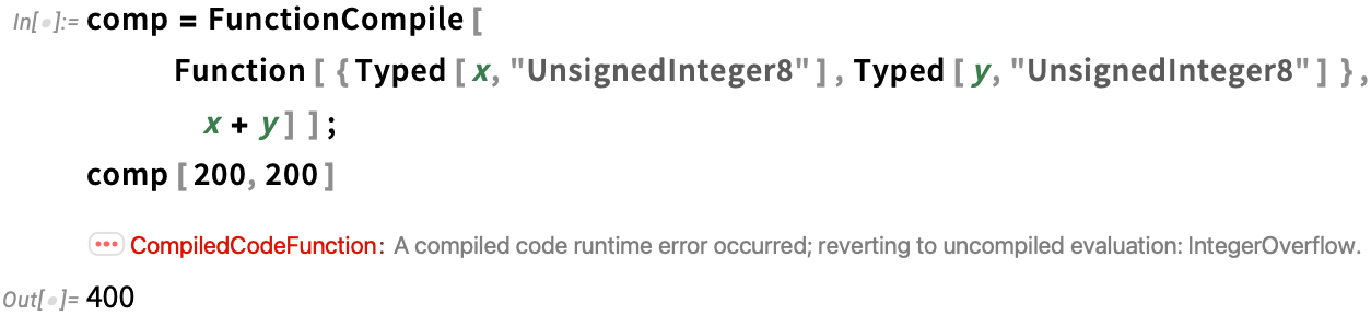
But in Version 14.1 there a new option CompilerRuntimeErrorAction that lets you specify an action to take (or, in general, a function to apply) whenever a runtime error occurs. A setting of None aborts the whole computation if there’s a runtime error:
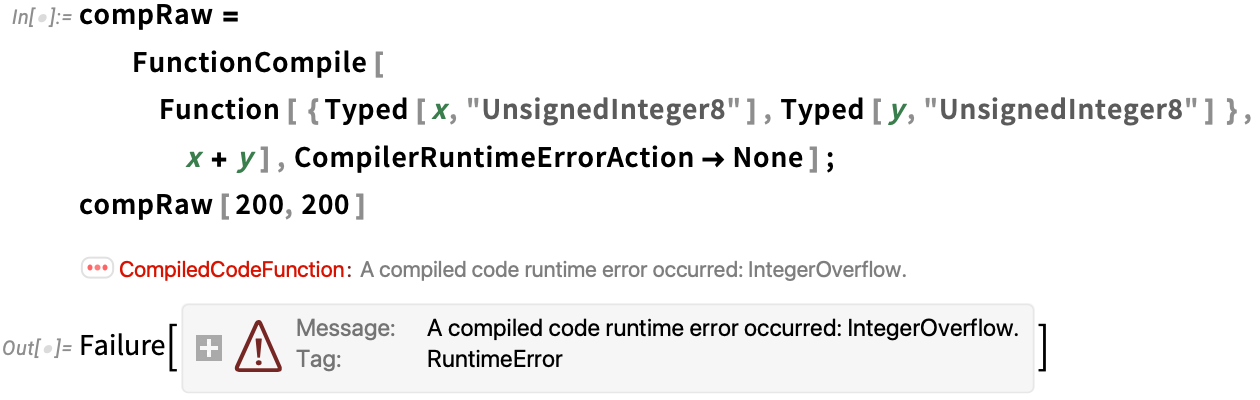
Even Smoother Integration with External Languages
Let’s say there’s some functionality you want to use, but the only implementation you have is in a package in some external language, like Python. Well, it’s now basically seamless to work with such functionality directly in the Wolfram Language—plugging into the whole symbolic framework and functionality of the Wolfram Language.
As a simple example, here’s a function that uses the Python package faker to produce a random sentence (which of course would also be straightforward to do directly in Wolfram Language):
The first time you run RandomSentence, the progress monitor will show you all sorts of messy things happening under the hood, as Python versions get loaded, dependencies get set up, and so on. But the point is that it’s all automatic, and so you don’t have to worry about it. And in the end, out pops the answer:

And if you run the function again, all the setup will already have been done, and the answer will pop out immediately:
An important piece of automation here is the conversion of data types. One of the great things about the Wolfram Language is that it has fully integrated symbolic representations for a very wide range of things—from videos to molecules to IP addresses. And when there are standard representations for these things in a language like Python, we’ll automatically convert to and from them.
But particularly with more sophisticated packages, there’ll be a need to let the package deal with its own “external objects” that are basically opaque to the Wolfram Language, but can be handled as atomic symbolic constructs there.
For example, let’s say we’ve started a Python external package chess (and, yes, there’s a paclet in the Wolfram Paclet Repository that has considerably more chess functionality):
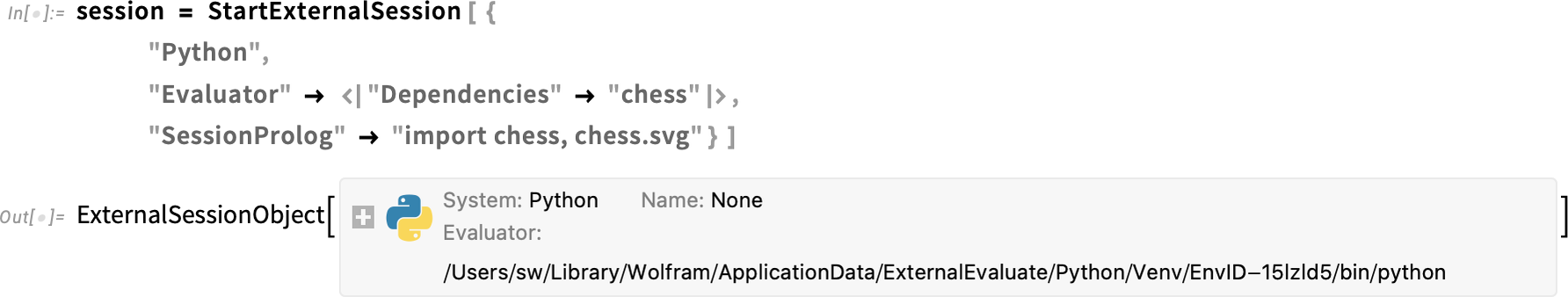
Now the state of a chessboard can be represented by an external object:
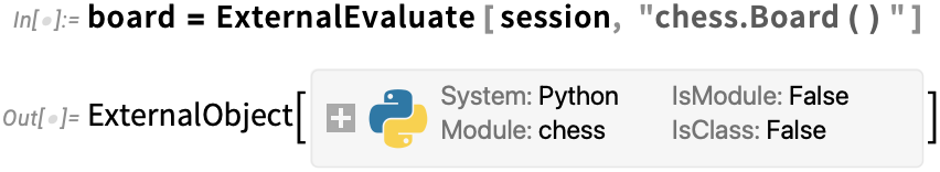
We can define a function to plot the board:
And now in Version 14.1 you can just pass your external object to the external function:
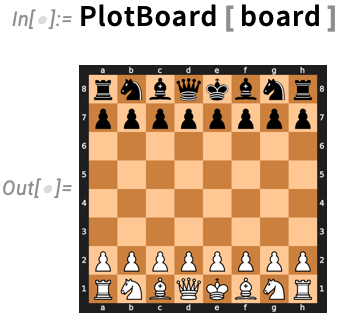
You can also directly extract attributes of the external object:
And you can call methods (here to make a chess move), changing the state of the external object:
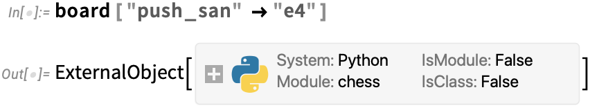
Here’s a plot of a new board configuration:
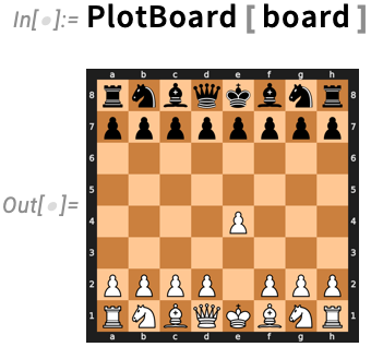
This computes all legal moves from the current position, representing them as external objects:
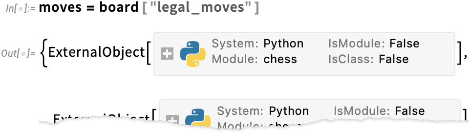
Here are UCI string representations of these:
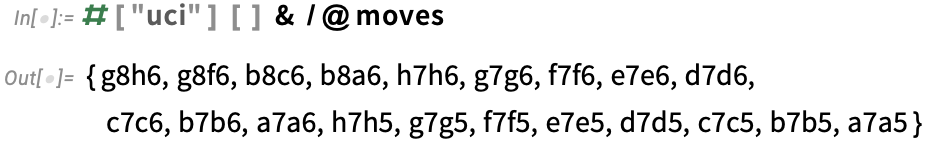
In what we’re doing here we’re immediately performing each external operation. But Version 14.1 introduces the construct ExternalOperation which lets you symbolically represent an external operation, and for example build up collections of such operations that can all be performed together in a single external evaluation. ExternalObject supports various built-in operations for each environment. So, for example, in Python we can use Call and GetAttribute to get the symbolic representation:
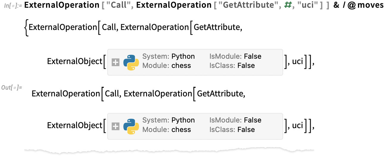
If we evaluate this, all these operations will get done together in the external environment:
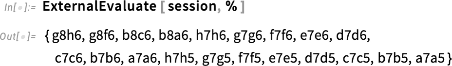
Standalone Wolfram Language Applications!
Let’s say you’re writing an application in pretty much any programming language—and inside it you want to call Wolfram Language functionality. Well, you could always do that by using a web API served from the Wolfram Cloud. And you could also do it locally by running the Wolfram Engine. But in Version 14.1 there’s something new: a way of integrating a standalone Wolfram Language runtime right into your application. The Wolfram Language runtime is a dynamic library that you link into your program, and then call using a C-based API. How big is the runtime? Well, it depends on what you want to use in the Wolfram Language. Because we now have the technology to prune a runtime to include only capabilities needed for particular Wolfram Language code. And the result is that adding the Wolfram Language will often increase the disk requirements of your application only by a remarkably small amount—like just a few hundred megabytes or even less. And, by the way, you can distribute the Wolfram runtime as an integrated part of an application, with its users not needing their own licenses to run it.
OK, so how does creating a standalone Wolfram-enabled application actually work? There’s a lot of software engineering (associated with the Wolfram Language runtime, how it’s called, etc.) under the hood. But at the level of the application programmer you only have to deal with our Standalone Applications SDK—whose interface is rather simple.
As an example, here’s the C code part of a standalone application that uses the Wolfram Language to identify what (human) language a piece of text is in. The program here takes a string of text on its command line, then runs the Wolfram Language LanguageIdentify function on it, and then prints a string giving the result:

If we ignore issues of pruning, etc. we can compile this program just with (and, yes, the file paths are necessarily a bit long):

Now we can run the resulting executable directly from the command line—and it’ll act just like any other executable, even though inside it’s got all the power of a Wolfram Language runtime:
![]()
If we look at the C program above, it basically begins just by starting the Wolfram Language runtime (using WLR_SDK_START_RUNTIME()). But then it takes the string (argv[1]) from the command line, embeds it in a Wolfram Language expression LanguageIdentify[string], evaluates this expression, and extracts a raw string from the result.
The functions, etc. that are involved here are part of the new Expression API supported by the Wolfram Language runtime dynamic library. The Expression API provides very clean capabilities for building up and taking apart Wolfram Language expressions from C. There are functions like wlr_Symbol("string") that form symbols, as well as macros like
How does the Expression API relate to WSTP? WSTP (“Wolfram Symbolic Transfer Protocol”) is our protocol for transferring symbolic expressions between processes. The Expression API, on the other hand, operates within a single process, providing the “glue” that connects C code to expressions in the Wolfram Language runtime.
One example of a real-world use of our new Standalone Applications technology is the LSPServer application that will soon be in full distribution. LSPServer started from a pure (though somewhat lengthy) Wolfram Language paclet that provides Language Server Protocol services for annotating Wolfram Language code in programs like Visual Studio Code. To build the LSPServer standalone application we just wrote a tiny C program that calls the paclet, then compiled this and linked it against our Standalone Applications SDK. Along the way (using tools that we’re planning to soon make available)—and based on the fact that only a small part of the full functionality of the Wolfram Language is needed to support LSPServer—we pruned the Wolfram Language runtime, in the end getting a complete LSPServer application that’s only about 170 MB in size, and that shows no outside signs of having Wolfram Language functionality inside.
And Yet More…
Is that all? Well, no. There’s more. Like new formatting of Root objects (yes, I was frustrated with the old one). Or like a new drag-and-drop-to-answer option for QuestionObject quizzes. Or like all the documentation we’ve added for new types of entities and interpreters.
In addition, there’s also the continual stream of new data that we’ve curated, or that’s flowed in real time into the Wolfram Knowledgebase. And beyond the core Wolfram Language itself, there’ve also been lots of functions added to the Wolfram Function Repository, lots of paclets added to the Wolfram Language Paclet Repository, not to mention new entries in the Wolfram Neural Net Repository, Wolfram Data Repository, etc.
Yes, as always it’s been a lot of work. But today it’s here, and we’re proud of it: Version 14.1!
Posted in: Mathematica, New Technology, Wolfram Language