And We’re Off and Running…
We recently wrapped up the four weeks of our first-ever “Physics track” Wolfram Summer School—and the results were spectacular! More than 30 projects potentially destined to turn into academic papers—reporting all kinds of progress on the Wolfram Physics Project.
When we launched the Wolfram Physics Project just three months ago one of the things I was looking forward to was seeing other people begin to seriously contribute to the project. Well, it turns out I didn’t have to wait long! Because—despite the pandemic and everything—things are already very much off and running!
Six weeks ago we made a list of questions we thought we were ready to explore in the Wolfram Physics Project. And in the past five weeks I’m excited to say that through projects at the Summer School lots of these are already well on their way to being answered. If we ever wondered whether there was a way for physicists (and physics students) to get involved in the project, we can now give a resounding answer, “yes”.
So what was figured out at the Summer School? I’m not going to get even close to covering everything here; that’ll have to await the finishing of papers (that I’ll be most interested to read!). But I’ll talk here about a few things that I think are good examples of what was done, and on which I can perhaps provide useful commentary.
I should explain that we’ve been doing our Wolfram Summer School for 18 years now (i.e. since just after the 2002 publication of A New Kind of Science), always focusing on having each student do a unique original project. This year—for the first time—we did the Summer School virtually, with 79 college/graduate/postdoc/… students from 21 countries around the world (and, yes, 13 time zones). We had 30 students officially on the “Physics track”, but at least 35 projects ended up being about the Wolfram Physics Project. (Simultaneous with the last two weeks of the Summer School we also had our High School Summer Camp, with another 44 students—and several physics projects.)
My most important role in the Summer School (and Summer Camp) is in defining projects. For the Physics track Jonathan Gorard was the academic director, assisted by some very able mentors and TAs. Given how new the Wolfram Physics Project is, there aren’t many people who yet know it well, but one of the things we wanted to achieve at the Summer School was to fix that!
Nailing Down Quantum Mechanics
One of the remarkable features of our models is that they basically imply the inevitability of quantum mechanics. But what is the precise correspondence between our models and all the traditional formalism of quantum mechanics? Some projects at the Summer School helped the ongoing process of nailing that down.
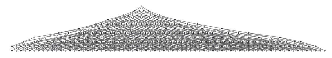
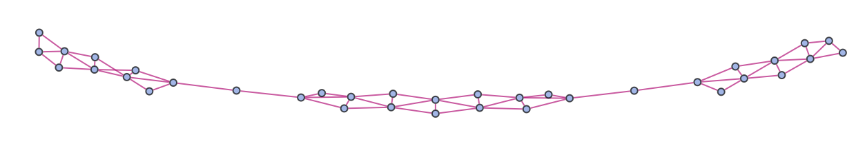
The starting point for any discussion of quantum mechanics in our models is the notion of multiway systems, and the concept that there can be many possible paths of evolution, represented by a multiway graph. The nodes in the multiway graph represent quantum (eigen)states. Common ancestry among these states defines entanglements between them. The branchial graph then in effect gives a map of the entanglements of quantum states—and in the large-scale limit one can think of this as corresponding to a “branchial space”:
The full picture of multiway systems for transformations between hypergraphs is quite complicated. But a key point that has become increasingly clear is that many of the core phenomena of quantum mechanics are actually quite generic to multiway systems, independent of the details of the underlying rules for transitions between states. And as a result, it’s possible to study quantum formalism just by looking at string substitution systems, without the full complexity of hypergraph transformations.
A quantum state corresponds to a collection of nodes in the multiway graph. Transitions between states through time can be studied by looking at the paths of bundles of geodesics through the multiway graph from the nodes of one state to another.
In traditional quantum formalism different states are assigned quantum amplitudes that are specified by complex numbers. One of our realizations has been that this “packaging” of amplitudes into complex numbers is quite misleading. In our models it’s much better to think about the magnitude and phase of the amplitude separately. The magnitude is obtained by looking at path weights associated with multiplicity of possible paths that reach a given state. The phase is associated with location in branchial space.
One of the most elegant results of our models so far is that geodesic paths in branchial space are deflected by the presence of relativistic energy density represented by the multiway causal graph—and therefore that the path integral of quantum mechanics is just the analog in branchial space of the Einstein equations in physical space.
To connect with the traditional formalism of quantum mechanics we must discuss how measurement works. The basic point is that to obtain a definite “measured result” we must somehow get something that no longer shows “quantum branches”. Assuming that our underlying system is causal invariant, this will eventually always “happen naturally”. But it’s also something that can be achieved by the way an observer (who is inevitably themselves embedded in the multiway system) samples the multiway graph. And as emphasized by Jonathan Gorard this is conveniently parametrized by thinking of the observer as effectively adding certain “completions” to the transition rules used to construct the multiway system.
It looks as if it’s then straightforward to understand things like the Born rule for quantum probabilities. (To project one state onto another involves a “rectangle” of transformations that have path weights corresponding to the product of those for the sides.) It also seems possible to understand things like destructive interference—essentially as the result of geodesics for different cases landing up at sufficiently distant points in branchial space that any “spanning completion” must pull in a large number of “randomly canceling” path weights.
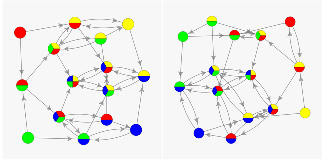
Local versus Global Multiway Systems
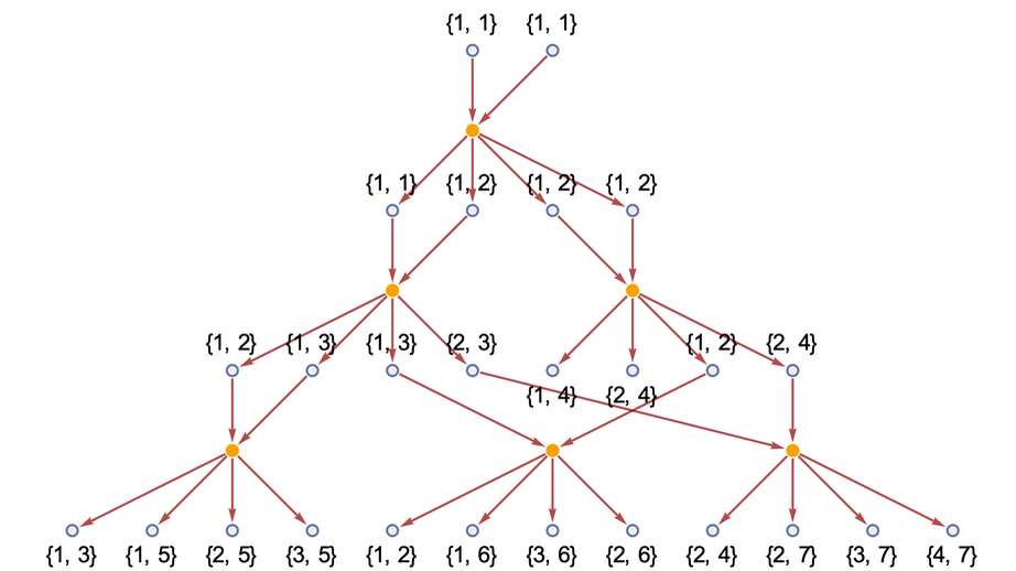
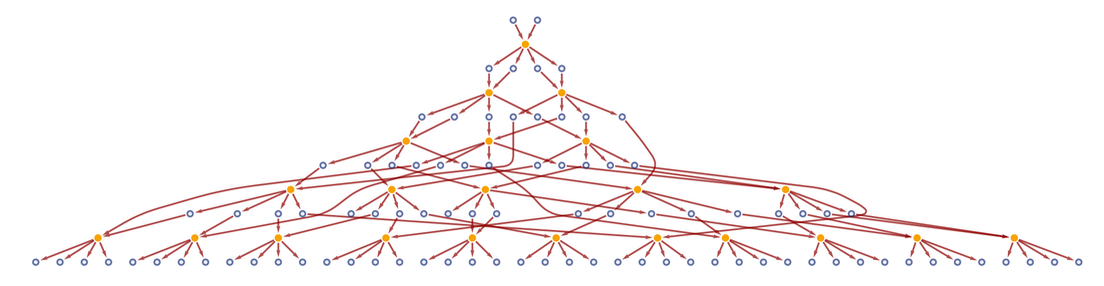
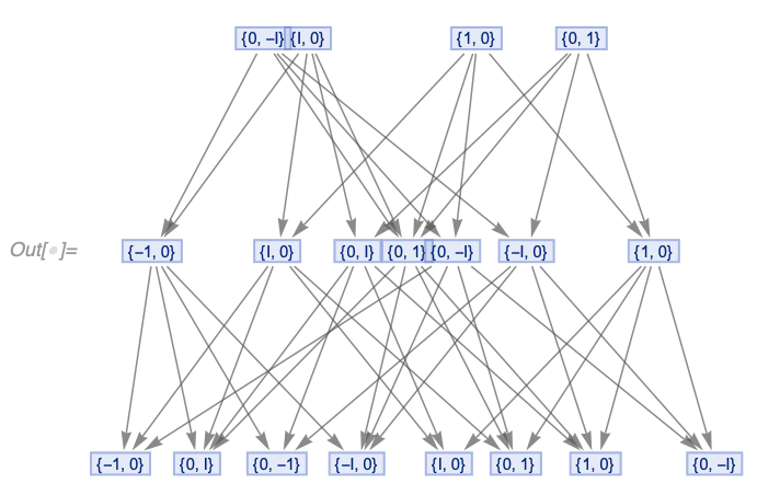
A standard “global” multiway system works by merging branches that lead to globally isomorphic hypergraphs. In Jonathan Gorard’s “completion interpretation of quantum mechanics”, some of these merges represent the results of applying rules that effectively get “added by the observer” as part of their interpretation of the universe. Max Piskunov has criticized the need to consider global hypergraph isomorphism (“Is one really going to compare complete universes?”)—and has suggested instead the idea of local multiway systems. He got the first implementation of local multiway systems done just in time for the Summer School.
Consider the rule:
{{x, y}, {x, z}} → {{x, z}, {x, w}, {y, w}, {z, w}}
Start from the initial state {{{1,1},{1,1}}}. Here’s its global multiway graph, showing both states and events:
✕
ResourceFunction["MultiwaySystem"][
 "WolframModel" -> {{{x, y}, {x, z}} -> {{x, z}, {x, w}, {y, w}, {z,
      w}}}, {{{1, 1}, {1, 1}}}, 3, "EvolutionEventsGraph",
 VertexSize -> 1]
|
But now imagine that we trace the fate of every single relation in each hypergraph, and show it as a separate node in our graph. What we get then is a local multiway system. In this case, here are the first few steps:
✕
ResourceFunction[
   "WolframModel"][{{x, y}, {x, z}} -> {{x, z}, {x, w}, {y, w}, {z,
     w}}, Automatic, 3]["ExpressionsEventsGraph",
 VertexLabels -> Automatic]
|
Continue for a few more steps:
✕
ResourceFunction[
   "WolframModel"][{{x, y}, {x, z}} -> {{x, z}, {x, w}, {y, w}, {z,
     w}}, Automatic, 5]["ExpressionsEventsGraph"]
|
If we look only at events, we get exactly the same causal graph as for the global multiway system:
✕
ResourceFunction[
   "WolframModel"][{{x, y}, {x, z}} -> {{x, z}, {x, w}, {y, w}, {z,
     w}}, Automatic, 5]["LayeredCausalGraph"]
|
But in the full local multiway graph every causal edge is “annotated” with the relation (or “expression”) that “carries” causal information between events.
In general, two events can be timelike, spacelike or branchlike separated. A local multiway system provides a definite criterion for distinguishing these. When two events are timelike separated, one can go from one to another by following a causal edge. When two events are spacelike separated, their most common ancestor in the local multiway system graph will be an event. But if they are branchlike separated, it will instead be an expression.
To reconstruct “complete states” (i.e. spatial hypergraphs) of the kind used in the global multiway system, one needs to assemble maximal collections of expressions that are spacelike separated (“maximal antichains” in poset jargon).
But so is the “underlying physics” of local multiway systems the same as global ones? In a global multiway system one talks about applying rules to the collections of expressions that exist in spatial hypergraphs. But in a local multiway system one just applies rules to arbitrary collections of expressions (or relations). And a big difference is that the expressions in these collections can lie not just at different places in a spatial hypergraph, but on different multiway branches. Or, in other words, the evolution of the universe can pick pieces from different potential “branches of history”.
This might sound like it’d lead to completely different results. But the remarkable thing is that it doesn’t—and instead global and multiway systems just seem to be different descriptions of what is ultimately the same thing. Let’s assume first that the underlying rules are causal invariant. Then in a global multiway system, branches must always reconverge. But this reconvergence means that even when there are states (and expressions) “on different branches” they can still be brought together into the same event, just like in a local multiway system. And when there isn’t immediately causal invariance, Jonathan’s “completion interpretation” posits that observers in effect add completions which lead to effective causal invariance, with the same reconvergence, and effective involvement of different branches in single events.
As Jonathan and Max debated global vs. local multiway systems I joked that it was a bit like Erwin Schrödinger debating Werner Heisenberg in the early days of quantum mechanics. And then we realized: actually it was just like that! Recall that in the Schrödinger picture of quantum mechanics, time evolution operators are fixed, but states evolve, whereas in the Heisenberg picture, states are fixed, but evolution operators evolve. Well, in a global multiway system one’s looking at complete states and seeing how they change as a result of the fixed set of events defined by the rules. But in a local multiway system one has a fixed basis of expressions, and then one’s looking at how the structure of the events that involve these expressions changes. So it’s just like the Schrödinger vs. Heisenberg pictures!
The Concept of Multispace
Right before the Summer School, I’d been doing quite a lot of work on what I was calling “multispace”. In a spatial hypergraph one’s representing the spatial relationships between elements. In a global multiway system one’s representing the branchial relationships between complete states. In a local multiway system spatial and branchial relationships are effectively mixed together.
So what is the analog of physical space when branchial relationships are included? I’m calling it multispace. In a case where there isn’t any branching—say an ordinary, deterministic Turing machine—multispace is just the same as ordinary space. But if there’s branching, it’s different.
Here’s an experiment I did just before the Summer School in the very simple case of a non-deterministic Turing machine:
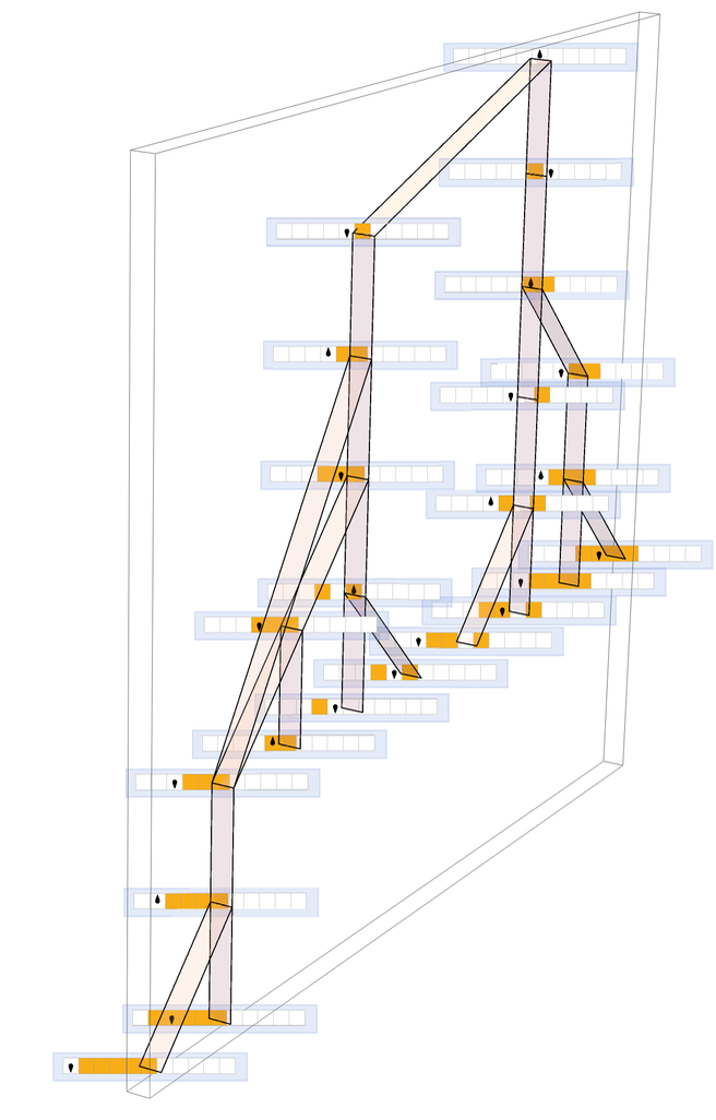
But I wasn’t really happy with this visualization; the most obvious structure is still the multiway system, and there are lots of “copies of space”, appearing in different states. What I wanted to figure out was how to visualize things so that ordinary space is somehow primary, and the branching is secondary. One could imagine that the elements of the system are basically laid out according to the relationships in ordinary space, merely “bulging out” in a different direction to represent branchial structure.
The practical problem is that branchial space may usually be much “bigger” than ordinary space, so the “bulging” may in effect “overpower” the ordinary spatial relationships. But one idea for visualizing multispace—explored by Nikolay Murzin at the Summer School—is to use machine-learning-like methods to create a 3D layout that shows spatial structure when viewed from one direction, and branchial structure when viewed from an orthogonal direction:
✕
ResourceFunction["MultispacePlot3D"][
 ResourceFunction["MultiwayTuringMachine"][{1507, 2506,
    3506}, {{1, 1, 0}, {0, 1, 0, 1}}, 4, ##] &, "Graph"]
|
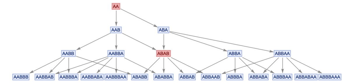
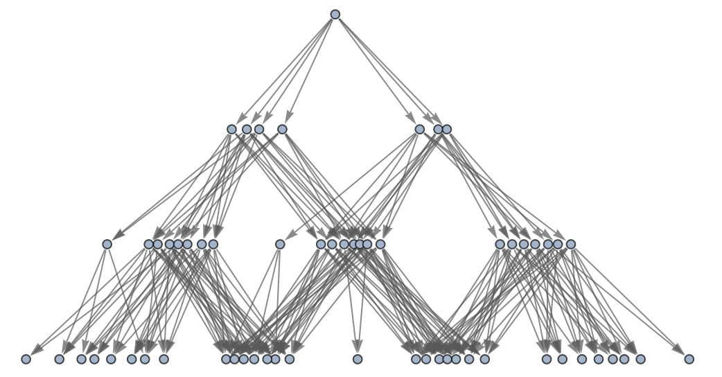
Generational States, the Ontological Basis and Bohmian Mechanics
In our models, multiway graphs represent all possible “quantum paths of evolution” for a system. But is there a way to pick out at least an approximation to a “classical-like path”? Yes–it’s a path consisting of a sequence of what we call “generational states”. And in going from one generational state to another, the idea is to carry out not just one event, as in the multiway graph, but a maximal set of spacelike separated events. In other words, instead of allowing different “quantum branches” containing different orderings of events, we’re insisting that a maximal set of consistent events are all done together.
Here’s an example. Consider the rule:
{A → AB, B → BBA}
Here’s a “classical-like path” made from generational states:
|
✕
ResourceFunction["GenerationalMultiwaySystem"][{"A" -> "AB",
  "B" -> "BBA"}, "AA", 3, "StatesGraph"]
|
These states must appear in the multiway graph, though it typically takes several events (i.e. several edges) to go from one to another (and in general there may be multiple “generational paths”, corresponding to multiple possible “classical-like paths” in a system):
✕
stripMetadata[expression_] :=
 If[Head[expression] === Rule, Last[expression], expression]; Graph[
 ResourceFunction["MultiwaySystem"][{"A" -> "AB",
   "B" -> "BBA"}, {"AA"}, 3, "StatesGraph"],
 VertexShapeFunction -> {Alternatives @@
     VertexList[
      ResourceFunction["GenerationalMultiwaySystem"][{"A" -> "AB",
        "B" -> "BBA"}, {"AA"}, 3, "StatesGraph"]] -> (Text[
       Framed[Style[stripMetadata[#2], Hue[0, 1, 0.48]],
        Background -> Directive[Opacity[.6], Hue[0, 0.45, 0.87]],
        FrameMargins -> {{2, 2}, {0, 0}}, RoundingRadius -> 0,
        FrameStyle ->
         Directive[Opacity[0.5],
          Hue[0, 0.52, 0.8200000000000001]]], #1, {0, 0}] &)}]
|
But what is the interpretation of generational states in previous discussions of quantum mechanics? Joseph Blazer’s project at the Summer School suggested that they are like an ontological basis.
In the standard formalism used for quantum mechanics one imagines that there are lots of quantum states that can form superpositions, etc.—and that classical results emerge only when measurements are done. But even from the earliest days of quantum mechanics (and rediscovered in the 1950s) there is an alternative formalism: so-called Bohmian mechanics, in which everything one considers is a “valid classical state”, but in which there are more elaborate rules of evolution than in the standard formalism.
Well, it seems as if generational states are just what Bohmian mechanics is talking about. The set of possible generational states can be thought of as forming an “ontological basis”, of states that “really can exist”, without any “quantum funny business”.
But what is the rule for evolution between generational states? One of the perhaps troubling features of Bohmian mechanics is that it implies correlations between spacelike separated events, or in other words, it implies that effects can propagate at arbitrarily high speeds.
But here’s the interesting thing: that’s just what happens in our generational states too! In our generational states, though, it isn’t some strange effect that seems to be arbitrarily added to the system: it’s simply a consequence of the consistency conditions we choose to impose in defining generational states.
Classic Quantum Systems and Effects
An obvious check on our models is to see them reproduce classic quantum systems and effects—and several projects at the Summer School were concerned with this. A crucial point (that I mentioned above) is that it’s becoming increasingly clear that at least most of these “classic quantum systems and effects” are quite generic features of our models—and of the multiway systems that appear in them. And this meant that many of the “quantum” projects at the Summer School could be done just in terms of string substitution systems, without having to deal with all the complexities of hypergraph rewriting.
Quantum Interference
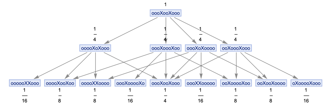
Hatem Elshatlawy, for example, explored quantum interference in our models. He got some nice results—which Jonathan Gorard managed to simplify to an almost outrageous extent.
Let’s imagine just having a string in which o represents “empty space”, and X represents the position of some quantum thing, like a photon. Then let’s have a simple sorting rule that represents the photon going either left or right (a kind of minimal Huygens’ principle):
{Xo → oX, oX → Xo}
Now let’s construct a multiway system starting from a state “oooXooXooo” that we can think of as corresponding to photons going through two “slits” a certain distance apart:
✕
ResourceFunction["MultiwaySystem"][{"Xo" -> "oX",
  "oX" -> "Xo"}, "oooXooXooo", 2, "StatesGraph",
 "IncludeStepNumber" -> True, "IncludeStateWeights" -> True,
 VertexLabels -> "VertexWeight",
 GraphLayout -> "LayeredDigraphEmbedding"]
|
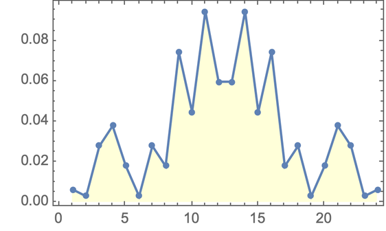
The merging of states that we see here is ultimately going to correspond to “quantum interference”. The path weights correspond to the magnitudes of the amplitudes of different states. But the question is: “What final state corresponds to what final photon position?”
Different final photon positions effectively correspond to different quantum phases for the photon. But in our models these quantum phases are associated with positions in branchial space. And to get an idea of what’s going on, we can just use the sorting order of strings to give a sense of relative positions in branchial space. (Because of the details of the setup, we need to just use the right-hand half of the strings, then symmetrically repeat them.)
If we now do this, and plot the values of the weights (here after 6 steps) this is what we get:
✕
Cell[CellGroupData[{
Cell[BoxData[
 RowBox[{
  RowBox[{"MultiwayDiffractionTest", "[",
   RowBox[{
   "rules_List", ",", "initialCondition_String", ",",
    "stepCount_Integer"}], "]"}], ":=",
  RowBox[{"Module", "[",
   RowBox[{
    RowBox[{"{",
     RowBox[{
     "allStatesList", ",", "finalStatesCount", ",", "weights", ",",
      "sortedWeights"}], "}"}], ",", "\[IndentingNewLine]",
    RowBox[{
     RowBox[{"allStatesList", "=",
      RowBox[{
       RowBox[{
       "ResourceFunction", "[", "\"\<MultiwaySystem\>\"", "]"}], "[",

       RowBox[{
       "rules", ",", "initialCondition", ",", "stepCount", ",",
        "\"\<AllStatesList\>\"", ",",
        RowBox[{"\"\<IncludeStateWeights\>\"", "\[Rule]", "True"}],
        ",",
        RowBox[{"VertexLabels", "\[Rule]", "\"\<VertexWeight\>\""}],
        ",",
        RowBox[{"\"\<IncludeStepNumber\>\"", "\[Rule]", "True"}]}],
       "]"}]}], ";", "\[IndentingNewLine]",
     RowBox[{"finalStatesCount", "=",
      RowBox[{"Length", "[",
       RowBox[{"Last", "[", "allStatesList", "]"}], "]"}]}], ";",
     "\[IndentingNewLine]",
     RowBox[{"weights", "=",
      RowBox[{
       RowBox[{
       "ResourceFunction", "[", "\"\<MultiwaySystem\>\"", "]"}], "[",

       RowBox[{
       "rules", ",", "initialCondition", ",", "stepCount", ",",
        "\"\<StateWeights\>\"", ",",
        RowBox[{"\"\<IncludeStateWeights\>\"", "\[Rule]", "True"}]}],
       "]"}]}], ";", "\[IndentingNewLine]",
     RowBox[{"sortedWeights", "=",
      RowBox[{"Join", "[",
       RowBox[{
        RowBox[{"Reverse", "[",
         RowBox[{"Take", "[",
          RowBox[{"weights", ",",
           RowBox[{"-",
            RowBox[{"Ceiling", "[",
             RowBox[{"finalStatesCount", "/", "2"}], "]"}]}]}], "]"}],
          "]"}], ",",
        RowBox[{"Take", "[",
         RowBox[{"weights", ",",
          RowBox[{"-",
           RowBox[{"Ceiling", "[",
            RowBox[{"finalStatesCount", "/", "2"}], "]"}]}]}],
         "]"}]}], "]"}]}], ";", "\[IndentingNewLine]",
     RowBox[{"Last", "/@", "sortedWeights"}]}]}], "]"}]}]], "Input"],

 Cell[BoxData[
 RowBox[{"ListLinePlot", "[",
  RowBox[{
   RowBox[{"MultiwayDiffractionTest", "[",
    RowBox[{
     RowBox[{"{",
      RowBox[{
       RowBox[{"\"\<Xo\>\"", "\[Rule]", "\"\<oX\>\""}], ",",
       RowBox[{"\"\<oX\>\"", "\[Rule]", "\"\<Xo\>\""}]}], "}"}], ",",
     " ", "\"\<oooXooXooo\>\"", ",", "6"}], "]"}], ",",
   RowBox[{"Mesh", "\[Rule]", "All"}], ",",
   RowBox[{"Frame", "\[Rule]", "True"}], ",",
   RowBox[{"Filling", "\[Rule]", "Axis"}], ",",
   RowBox[{"FillingStyle", "->", "LightYellow"}]}], "]"}]], "Input"]
|
Amazingly, this is starting to look a bit like a diffraction pattern. Let’s try “increasing the slit spacing”—by using the initial string “ooooooooXoooXoooooooo”. Now the multiway graph has the form
✕
LayeredGraphPlot[
 ResourceFunction["MultiwaySystem"][{"Xo" -> "oX", "oX" -> "Xo"},
  "ooooooooXoooXoooooooo", 10, "EvolutionGraphStructure"]]
|
and plotting the weights we get
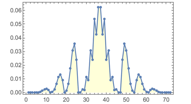
✕
ListLinePlot[
 MultiwayDiffractionTest[{"Xo" -> "oX", "oX" -> "Xo"},
  "ooooooooXoooXoooooooo", 10], Mesh -> All, Frame -> True,
 Filling -> Axis, FillingStyle -> LightYellow]
|
which is stunningly similar to the standard quantum mechanics result
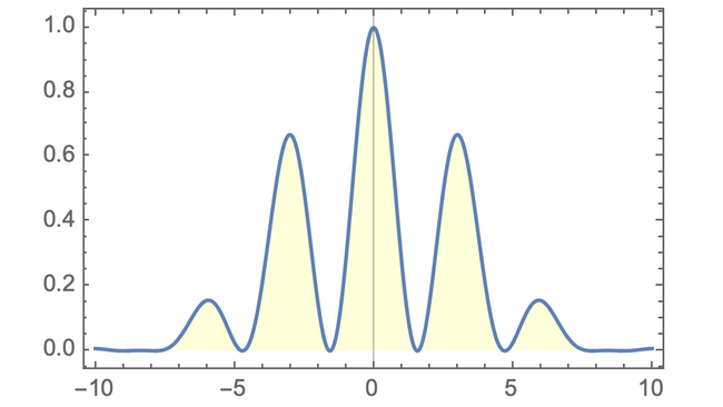
✕
Plot[((1/2)*ChebyshevU[1, Cos[x]]*Sinc[0.35*x])^2, {x, -10, 10},
 Filling -> Axis, FillingStyle -> LightYellow, Frame -> True]
|
complete with the expected destructive interference away from the central peak.
Computing the corresponding branchial graph we get
✕
ResourceFunction["MultiwaySystem"][{"Xo" -> "oX",
  "oX" -> "Xo"}, "ooooooooXoooXoooooooo", 10, \
"BranchialGraphStructure"]
|
which in effect shows the “concentrations of amplitude” into different parts of branchial space (AKA peaks in different regions of quantum phase).
(In a sense the fact that this all works is “unsurprising”, since in effect we’re just implementing a discrete version of Huygens’ principle. But it’s very satisfying to see everything come together.)
The Quantum Harmonic Oscillator
The quantum harmonic oscillator is one of the first kinds of quantum systems a typical quantum mechanics textbook will discuss. But how does the quantum harmonic oscillator work in our models? Patrick Geraghty’s project at the Summer School began the process of figuring it out.
A classical harmonic oscillator basically has something going back and forth in a certain region at a sequence of possible frequencies. The quantum harmonic oscillator picks up the same “modes”, but now represents them just as quantum eigenstates of a certain energy. In our models it’s actually possible to go back to something very close to the classical picture. We can set up a string substitution system in which something (here B or C) goes back and forth in a string of fixed length:
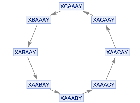
✕
ResourceFunction["MultiwaySystem"][{"BA" -> "AB", "BY" -> "CY",
  "AC" -> "CA", "XC" -> "XB"}, {"XBAAAY"}, 10, "StatesGraph"]
|
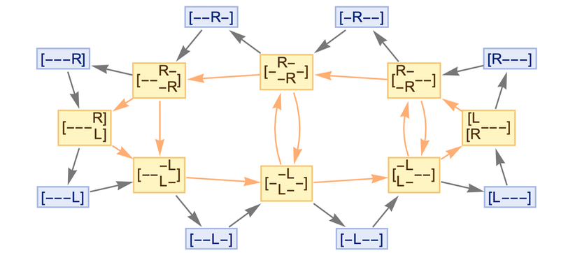
We can make it a bit more obvious what’s going on by changing the characters in the strings:

✕
ResourceFunction["MultiwaySystem"][{"R-" -> "-R", "R]" -> "L]",
  "-L" -> "L-", "[L" -> "[R"}, {"[R---]"}, 10, "StatesGraph"]
|
And it’s clear that this system will always go in a periodic cycle. If we were thinking about spacetime and relativity, it might trouble us that we’ve created a closed timelike curve, in which the future merges with the past. But that’s basically what we’re forced into by the idealization of a quantum harmonic oscillator.
Recall that in our models energy is associated with the flux of causal edges. Well, in this model of the harmonic oscillator, we can immediately figure out the causal edges:
✕
ResourceFunction["MultiwaySystem"][{"R-" -> "-R", "R]" -> "L]",
  "-L" -> "L-", "[L" -> "[R"}, {"[R---]"}, 10, "EvolutionCausalGraph"]
|
And we can see that as we change the length of the string, the number of causal edges (i.e. the energy) will linearly increase, as we’d expect for a quantum harmonic oscillator:
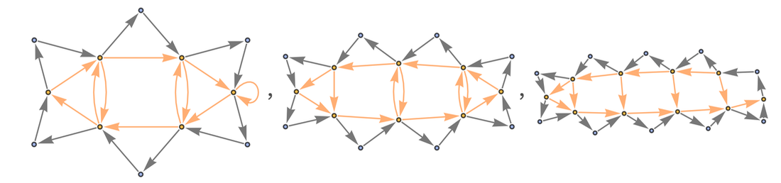
✕
Table[ResourceFunction["MultiwaySystem"][{"R-" -> "-R", "R]" -> "L]",
   "-L" -> "L-", "[L" -> "[R"}, {"[R" <> StringRepeat["-", n] <> "]"},
   10, "EvolutionCausalGraphStructure"], {n, 2, 4}]
|
Oh, and there’s even zero-point energy:
![Table[ResourceFunction["MultiwaySystem"]](https://content.wolfram.com/sites/43/2020/07/wss0731img29.png)
✕
Table[ResourceFunction["MultiwaySystem"][{"R-" -> "-R", "R]" -> "L]",
   "-L" -> "L-", "[L" -> "[R"}, {"[R" <> StringRepeat["-", n] <> "]"},
   10, "EvolutionCausalGraphStructure"], {n, 0, 2, 4}]
|
There’s a lot more to figure out even about the quantum harmonic oscillator, but this is a start.
Quantum Teleportation
One of the strange, but characteristic, phenomena that’s known to occur in quantum mechanics is what’s called quantum teleportation. In a physical quantum teleportation experiment, one creates a quantum-entangled pair of particles, then lets them travel apart. But now as soon as one measures the state of one of these particles, one immediately knows something about the state of the other particle—even though there hasn’t been time to get a light signal from that other particle.
At the Summer School, Taufiq Murtadho figured out a rather elegant way to understand this phenomenon in our models. I’ll not go through the details here, but here’s a representation of a key part of the construction:
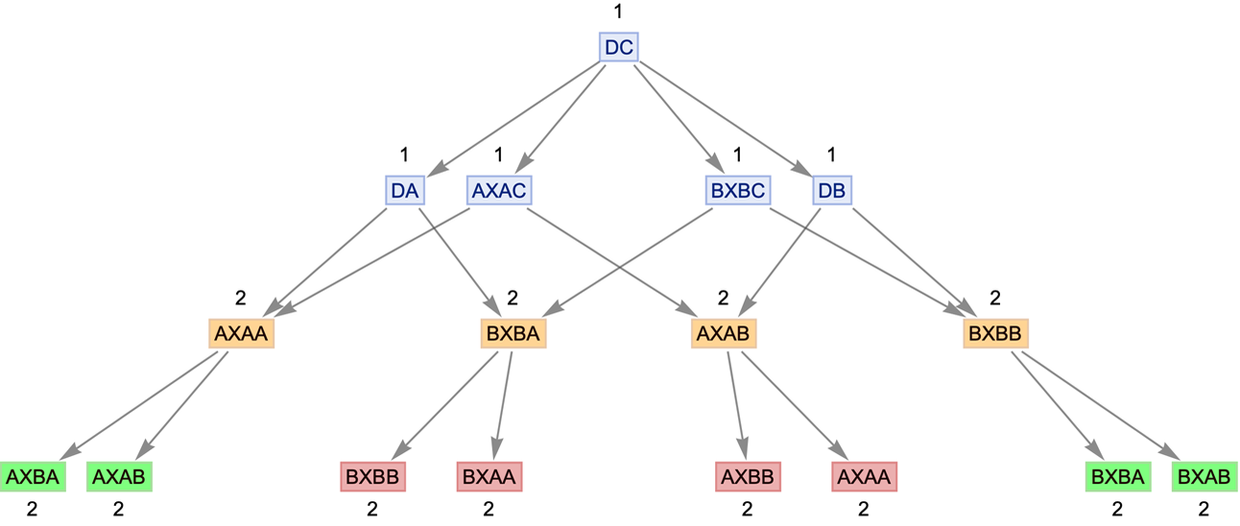
✕
Cell[CellGroupData[{
						Cell[BoxData[{
 RowBox[{
  RowBox[{"rule", " ", "=", " ",
   RowBox[{"{",
    RowBox[{
     RowBox[{"\"\<D\>\"", "\[Rule]", " ", "\"\<AXA\>\""}], ",",
     RowBox[{"\"\<D\>\"", "\[Rule]", " ", "\"\<BXB\>\""}], ",",
     RowBox[{"\"\<C\>\"", "\[Rule]", " ", "\"\<A\>\""}], ",",
     RowBox[{"\"\<C\>\"", "\[Rule]", " ", "\"\<B\>\""}]}], "}"}]}],
  ";"}], "\[IndentingNewLine]",
 RowBox[{
  RowBox[{"InitialState", " ", "=", "\"\<DC\>\""}],
  ";"}], "\[IndentingNewLine]",
 RowBox[{
  RowBox[{"BellCompletion", "=",
   RowBox[{"{",
    RowBox[{
     RowBox[{"\"\<BA\>\"", "\[Rule]", " ", "\"\<AA\>\""}], ",", " ",
     RowBox[{"\"\<AA\>\"", "\[Rule]", " ", "\"\<BA\>\""}], ",",
     RowBox[{"\"\<BA\>\"", "\[Rule]", " ", "\"\<BB\>\""}], ",",
     RowBox[{"\"\<BB\>\"", "\[Rule]", " ", "\"\<BA\>\""}], ",", " ",
     RowBox[{"\"\<AB\>\"", "\[Rule]", " ", "\"\<AA\>\""}], ",",
     RowBox[{"\"\<AA\>\"", "\[Rule]", " ", "\"\<AB\>\""}], ",", " ",
     RowBox[{"\"\<AB\>\"", "\[Rule]", " ", "\"\<BB\>\""}], ",",
     RowBox[{"\"\<BB\>\"", "\[Rule]", " ", "\"\<AB\>\""}]}], "}"}]}],
  ";"}]}], "Input"],

  Cell[BoxData[
 RowBox[{
  RowBox[{"(*",
   RowBox[{
   "Function", " ", "to", " ", "draw", " ", "the", " ", "graph", " ",
    "with", " ", "annotation"}], "*)"}], "\[IndentingNewLine]",
  RowBox[{
   RowBox[{
    RowBox[{"DrawGraph", "[", "]"}], ":=",
    RowBox[{"Module", "[",
     RowBox[{
      RowBox[{"{",
       RowBox[{"a", ",", "b", ",", "c"}], "}"}], ",",
      "\[IndentingNewLine]",
      RowBox[{"(*",
       RowBox[{
       "Selecting", " ", "the", " ", "vertices", " ", "to", " ", "be",
         " ", "colored"}], "*)"}], "\[IndentingNewLine]",
      RowBox[{
       RowBox[{"EvolVertexList", " ", "=", " ",
        RowBox[{"VertexList", "[",
         RowBox[{
          RowBox[{
          "ResourceFunction", "[", "\"\<MultiwaySystem\>\"", "]"}],
          "[",
          RowBox[{
           RowBox[{"Join", "[",
            RowBox[{"rule", ",", "BellCompletion"}], "]"}], ",",
           "InitialState", ",", "4", ",", "\"\<EvolutionGraph\>\""}],
          "]"}], "]"}]}], ";", "\[IndentingNewLine]",
       RowBox[{"TeleportInitState", " ", "=", " ",
        RowBox[{"FilterRules", "[",
         RowBox[{"EvolVertexList", ",", "2"}], "]"}]}], ";",
       "\[IndentingNewLine]",
       RowBox[{"BellVertex1", " ", "=",
        RowBox[{"Map", "[",
         RowBox[{
          RowBox[{
           RowBox[{"3", "\[Rule]", " ", "#"}], "&"}], ",",
          RowBox[{"Flatten", "[",
           RowBox[{"StringCases", "[",
            RowBox[{
             RowBox[{
              RowBox[{"FilterRules", "[",
               RowBox[{"EvolVertexList", ",", "3"}], "]"}], "/.",
              RowBox[{
               RowBox[{"Rule", "[",
                RowBox[{"a_", ",", "b_"}], "]"}], "\[RuleDelayed]",
               "b"}]}], ",",
             RowBox[{"{",
              RowBox[{
               RowBox[{"__", "~~", "\"\<AA\>\""}], ",",
               RowBox[{"__", "~~", "\"\<BB\>\""}]}], "}"}]}], "]"}],
           "]"}]}], "]"}]}], ";", "\[IndentingNewLine]",
       RowBox[{"BellVertex2", " ", "=",
        RowBox[{"Map", "[",
         RowBox[{
          RowBox[{
           RowBox[{"3", "\[Rule]", " ", "#"}], "&"}], ",",
          RowBox[{"Flatten", "[",
           RowBox[{"StringCases", "[",
            RowBox[{
             RowBox[{
              RowBox[{"FilterRules", "[",
               RowBox[{"EvolVertexList", ",", "3"}], "]"}], "/.",
              RowBox[{
               RowBox[{"Rule", "[",
                RowBox[{"a_", ",", "b_"}], "]"}], "\[RuleDelayed]",
               "b"}]}], ",",
             RowBox[{"{",
              RowBox[{
               RowBox[{"__", "~~", "\"\<AB\>\""}], ",",
               RowBox[{"__", "~~", "\"\<BA\>\""}]}], "}"}]}], "]"}],
           "]"}]}], "]"}]}], ";", "\[IndentingNewLine]",
       RowBox[{
        RowBox[{"stripMetadata", "[", "expression_", "]"}], ":=",
        RowBox[{"If", "[",
         RowBox[{
          RowBox[{
           RowBox[{"Head", "[", "expression", "]"}], "===", "Rule"}],
          ",",
          RowBox[{"Last", "[", "expression", "]"}], ",",
          "expression"}], "]"}]}], ";", "\[IndentingNewLine]",
       RowBox[{"(*",
        RowBox[{"Coloring", " ", "BellVertex1"}], "*)"}],
       "\[IndentingNewLine]",
       RowBox[{"a", " ", "=",
        RowBox[{"Graph", "[",
         RowBox[{
          RowBox[{
           RowBox[{
           "ResourceFunction", "[", "\"\<MultiwaySystem\>\"", "]"}],
           "[",
           RowBox[{
            RowBox[{"Join", "[",
             RowBox[{"rule", ",", "BellCompletion"}], "]"}], ",",
            "InitialState", ",", "3", ",", "\"\<EvolutionGraph\>\"",
            ",",
            RowBox[{
            "\"\<IncludeStatePathWeights\>\"", "\[Rule]", " ",
             "True"}], ",",
            RowBox[{
            "VertexLabels", "\[Rule]", " ",
             "\"\<VertexWeight\>\""}]}], "]"}], ",",
          InterpretationBox[
           DynamicModuleBox[{Typeset`open = False},
            TemplateBox[{"Expression",
              RowBox[{"Rule", "[",
                DynamicBox[
                 FEPrivate`FrontEndResource[
                 "FEBitmaps", "IconizeEllipsis"]], "]"}],
              GridBox[{{
                 ItemBox[
                  RowBox[{
                    TagBox["\"Byte count: \"", "IconizedLabel"],
                    "\[InvisibleSpace]",
                    TagBox["1776", "IconizedItem"]}]]}},
               GridBoxAlignment -> {"Columns" -> {{Left}}},
               DefaultBaseStyle -> "Column",
               GridBoxItemSize -> {
                "Columns" -> {{Automatic}}, "Rows" -> {{Automatic}}}],
              Dynamic[Typeset`open]},
             "IconizedObject"]],

           VertexShapeFunction -> {
            Apply[Alternatives, $CellContext`BellVertex1] -> (Text[
               Framed[
                Style[
                 $CellContext`stripMetadata[#2],
                 Hue[0, 1, 0.1]], Background -> Directive[
                  Opacity[0.6],
                  Hue[0, 0.45, 0.87]],
                FrameMargins -> {{2, 2}, {0, 0}}, RoundingRadius -> 0,
                 FrameStyle -> Directive[
                  Opacity[0.5],
                  Hue[0, 0.52, 0.8200000000000001]]], #, {0, 0}]& )},
           SelectWithContents->True,
           Selectable->False]}], "]"}]}], ";", "\[IndentingNewLine]",

       RowBox[{"(*",
        RowBox[{"Coloring", " ", "BellVertex2"}], "*)"}],
       "\[IndentingNewLine]",
       RowBox[{"b", " ", "=", " ",
        RowBox[{"Graph", "[",
         RowBox[{"a", ",",
          RowBox[{"VertexShapeFunction", "\[Rule]",
           RowBox[{"{",
            RowBox[{
             RowBox[{"Alternatives", "@@", "BellVertex2"}], "\[Rule]",
             RowBox[{"(",
              RowBox[{
               RowBox[{"Text", "[",
                RowBox[{
                 RowBox[{"Framed", "[",
                  RowBox[{
                   RowBox[{"Style", "[",
                    RowBox[{
                    RowBox[{"stripMetadata", "[", "#2", "]"}], ",",
                    RowBox[{"Hue", "[",
                    RowBox[{"0", ",", "1", ",", "0.1"}], "]"}]}],
                    "]"}], ",", "\[IndentingNewLine]",
                   RowBox[{"Background", "\[Rule]",
                    RowBox[{"Directive", "[",
                    RowBox[{
                    RowBox[{"Opacity", "[", ".6", "]"}], ",",
                    RowBox[{"Hue", "[",
                    RowBox[{
                    RowBox[{"1", "/", "3"}], ",", "1", ",", "1", ",",
                    ".5"}], "]"}]}], "]"}]}], ",",
                   InterpretationBox[
                    DynamicModuleBox[{Typeset`open = False},
                    TemplateBox[{"Expression", "SequenceIcon",
                    GridBox[{{
                    ItemBox[
                    RowBox[{
                    TagBox["\"Head: \"", "IconizedLabel"],
                    "\[InvisibleSpace]",
                    TagBox["Sequence", "IconizedItem"]}]]}, {
                    ItemBox[
                    RowBox[{
                    TagBox["\"Length: \"", "IconizedLabel"],
                    "\[InvisibleSpace]",
                    TagBox["3", "IconizedItem"]}]]}, {
                    ItemBox[
                    RowBox[{
                    TagBox["\"Byte count: \"", "IconizedLabel"],
                    "\[InvisibleSpace]",
                    TagBox["712", "IconizedItem"]}]]}},
                    GridBoxAlignment -> {"Columns" -> {{Left}}},
                    DefaultBaseStyle -> "Column",
                    GridBoxItemSize -> {
                    "Columns" -> {{Automatic}},
                    "Rows" -> {{Automatic}}}],
                    Dynamic[Typeset`open]},
                    "IconizedObject"]],
                    Sequence[
                    FrameMargins -> {{2, 2}, {0, 0}}, RoundingRadius ->
                    0, FrameStyle -> Directive[
                    Opacity[0.5],
                    Hue[0, 0.1, 0.8200000000000001]]],
                    SelectWithContents->True,
                    Selectable->False]}], "]"}], ",", "#1", ",",
                 RowBox[{"{",
                  RowBox[{"0", ",", "0"}], "}"}]}], "]"}], "&"}],
              ")"}]}], "}"}]}]}], "]"}]}], ";", "\[IndentingNewLine]",
       RowBox[{"(*",
        RowBox[{
        "Coloring", " ", "the", " ", "initial", " ", "teleportation",
         " ", "state"}], "*)"}], "\[IndentingNewLine]",
       RowBox[{"c", " ", "=", " ",
        RowBox[{"Graph", "[",
         RowBox[{"b", ",",
          RowBox[{"VertexShapeFunction", "\[Rule]",
           RowBox[{"{",
            RowBox[{
             RowBox[{"Alternatives", "@@", "TeleportInitState"}],
             "\[Rule]",
             RowBox[{"(",
              RowBox[{
               RowBox[{"Text", "[",
                RowBox[{
                 RowBox[{"Framed", "[",
                  RowBox[{
                   RowBox[{"Style", "[",
                    RowBox[{
                    RowBox[{"stripMetadata", "[", "#2", "]"}], ",",
                    RowBox[{"Hue", "[",
                    RowBox[{"0", ",", "1", ",", "0.1"}], "]"}]}],
                    "]"}], ",", "\[IndentingNewLine]",
                   InterpretationBox[
                    DynamicModuleBox[{Typeset`open = False},
                    TemplateBox[{"Expression", "SequenceIcon",
                    GridBox[{{
                    ItemBox[
                    RowBox[{
                    TagBox["\"Head: \"", "IconizedLabel"],
                    "\[InvisibleSpace]",
                    TagBox["Sequence", "IconizedItem"]}]]}, {
                    ItemBox[
                    RowBox[{
                    TagBox["\"Length: \"", "IconizedLabel"],
                    "\[InvisibleSpace]",
                    TagBox["4", "IconizedItem"]}]]}, {
                    ItemBox[
                    RowBox[{
                    TagBox["\"Byte count: \"", "IconizedLabel"],
                    "\[InvisibleSpace]",
                    TagBox["1008", "IconizedItem"]}]]}},
                    GridBoxAlignment -> {"Columns" -> {{Left}}},
                    DefaultBaseStyle -> "Column",
                    GridBoxItemSize -> {
                    "Columns" -> {{Automatic}},
                    "Rows" -> {{Automatic}}}],
                    Dynamic[Typeset`open]},
                    "IconizedObject"]],
                    Sequence[Background -> Directive[
                    Opacity[0.6],
                    Hue[0.1, 0.7, 3]],
                    FrameMargins -> {{2, 2}, {0, 0}}, RoundingRadius ->
                    0, FrameStyle -> Directive[
                    Opacity[0.5],
                    Hue[0, 0.1, 0.8200000000000001]]],
                    SelectWithContents->True,
                    Selectable->False]}], "]"}], ",", "#1", ",",
                 RowBox[{"{",
                  RowBox[{"0", ",", "0"}], "}"}]}], "]"}], "&"}],
              ")"}]}], "}"}]}]}], "]"}]}]}]}], "]"}]}],
   "\[IndentingNewLine]",
   RowBox[{"(*",
    RowBox[{"Run", " ", "the", " ", "function"}], "*)"}],
   "\[IndentingNewLine]",
   RowBox[{"DrawGraph", "[", "]"}]}]}]], "Input"]
}, Open  ]]
|
A feature of quantum teleportation is that even though the protocol seems to be transmitting information faster than light, that isn’t really what’s happening when one traces everything through. And what Taufiq found is that in our models the multiway causal graph reveals how this works. In essence, the “teleportation” happens through causal edges that connect branchlike separated states—but these edges cannot transmit an actual measurable message.
Quantum Computing
How do we tell if our models correctly reproduce something like quantum computing? One approach is what I call “proof by compilation”. Just take a standard description of something—here quantum computing—and then systematically “compile” it to a representation in terms of our models.
Just before the Summer School, Jonathan Gorard put a function into the Wolfram Function Repository called QuantumToMultiwaySystem, which takes a description of a quantum circuit and “compiles it” to one of our multiway systems:

For example, here’s a Pauli-Z gate compiled to the rules for a multiway system:

✕
ResourceFunction[
ResourceObject[
Association[
   "Name" -> "QuantumToMultiwaySystem",
    "ShortName" -> "QuantumToMultiwaySystem",
    "UUID" -> "11c8aade-c41e-481e-85c0-10424fa9edbd",
    "ResourceType" -> "Function", "Version" -> "1.0.0",
    "Description" -> "Simulate a quantum evolution as a multiway \
system", "RepositoryLocation" -> URL[
     "https://www.wolframcloud.com/objects/resourcesystem/api/1.0"],
    "SymbolName" -> "FunctionRepository`$\
337d322381db46d0b0c8103362842dec`QuantumToMultiwaySystem",
    "FunctionLocation" -> CloudObject[
     "https://www.wolframcloud.com/obj/34b943dd-88a8-423c-a3d3-\
07922920160a"]], ResourceSystemBase -> Automatic]][<|
  "Operator" -> {{1, 0}, {0, -1}}, "Basis" -> {{1, 0}, {0, 1}}|>]
|
Here now is the result of starting with a superposition of states and running two steps of root-NOT gates:
✕
ResourceFunction[
ResourceObject[
Association[
   "Name" -> "QuantumToMultiwaySystem",
    "ShortName" -> "QuantumToMultiwaySystem",
    "UUID" -> "11c8aade-c41e-481e-85c0-10424fa9edbd",
    "ResourceType" -> "Function", "Version" -> "1.0.0",
    "Description" -> "Simulate a quantum evolution as a multiway \
system", "RepositoryLocation" -> URL[
     "https://www.wolframcloud.com/objects/resourcesystem/api/1.0"],
    "SymbolName" -> "FunctionRepository`$\
337d322381db46d0b0c8103362842dec`QuantumToMultiwaySystem",
    "FunctionLocation" -> CloudObject[
     "https://www.wolframcloud.com/obj/34b943dd-88a8-423c-a3d3-\
07922920160a"]], ResourceSystemBase -> Automatic]][<|
  "Operator" -> {{1 + I, 1 - I}, {1 - I, 1 + I}},
  "Basis" -> {{1, 0}, {0, 1}}|>, {1 + I,
  1 - I}, 2, "EvolutionGraphFull"]
|
And, yes, we can understand entanglements through branchial graphs, etc.:

✕
ResourceFunction[
ResourceObject[
Association[
   "Name" -> "QuantumToMultiwaySystem",
    "ShortName" -> "QuantumToMultiwaySystem",
    "UUID" -> "11c8aade-c41e-481e-85c0-10424fa9edbd",
    "ResourceType" -> "Function", "Version" -> "1.0.0",
    "Description" -> "Simulate a quantum evolution as a multiway \
system", "RepositoryLocation" -> URL[
     "https://www.wolframcloud.com/objects/resourcesystem/api/1.0"],
    "SymbolName" -> "FunctionRepository`$\
337d322381db46d0b0c8103362842dec`QuantumToMultiwaySystem",
    "FunctionLocation" -> CloudObject[
     "https://www.wolframcloud.com/obj/34b943dd-88a8-423c-a3d3-\
07922920160a"]], ResourceSystemBase -> Automatic]][<|
  "Operator" -> {{1 + I, 1 - I}, {1 - I, 1 + I}},
  "Basis" -> {{1, 0}, {0, 1}}|>, {1 + I, 1 - I}, 2, "BranchialGraph"]
|
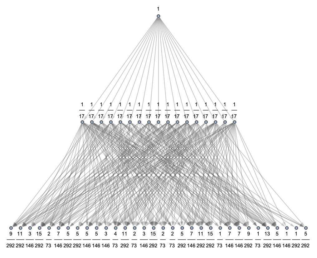
But, OK, if we can do this kind of compilation, what happens if we compile a famous quantum algorithm, like Shor’s algorithm for factoring integers, to a multiway system? At the Summer School, Yoav Rabinovich looked at this, working with Jack Heimrath and Jonathan Gorard. The whole of Shor’s algorithm is pretty messy, with lots of not-very-quantum parts. But the core of factoring an integer n is to do a quantum Fourier transform on Mod[a^Range[n],n], and then to do measurements on the resulting superposition of states and detect peaks.
Here’s a version of the quantum Fourier transform involved in factoring the integer n = 6, converted to one of our multiway systems:
And, yes, there’s a lot going on here, but at least it’s happening “in parallel” in different branches of the quantum evolution—in just a few time steps. But the result here is just a superposition of quantum states; to actually find “the answer” we have to do measurements to find which quantum states have the highest amplitude, or largest path weight.
In the usual formalism of quantum mechanics, we’d just talk about “doing the measurement”; we wouldn’t discuss what goes on “inside the measurement”. But in our model we can analyze the actual process of measurement. And at least in Jonathan’s “completion interpretation” we can say that the measurement is achieved by a multiway system in which the observer effectively defines completions that merge branches:
We’ve included path weights here, and “the answer” can effectively be read off by asking where in branchial space the maximum path weight occurs. But notice that lots of multiway edges (or events) had to be added to get the measurement done; that’s effectively the “cost of measurement” as revealed in our model.
So now the obvious question is: “How does this scale as one increases the number n? Including measurement, does the quantum computation ultimately succeed in factoring n in a polynomial number of steps?”
We don’t yet know the answer to this—but we’ve now more or less got the wherewithal to figure it out.
Here’s the basic picture. When we “do a quantum computation” we get to use the parallelism of having many different “threads” spread across branchial space. But when we want to measure what comes out, we have to “corral” all these threads back together to get a definite “observable” result. And the question is whether in the end we come out ahead compared to doing the purely classical computation.
I have to say that I’ve actually wondered about this for a very long time. And in fact, back in the early 1980s, when Richard Feynman and I worked on quantum computing, one of the main things we talked about was the “cost of measurement”. As an example, we looked at the “null” quantum computation of generating “random numbers” (e.g. from a process like radioactive decay)—and we ended up suspecting that there would be inevitable bounds on the “minimum cost of measurement”.
So it wouldn’t surprise me at all if in the end the “cost of measurement” wiped out any gains from “quantum parallelism”. But we don’t yet know for sure, and it will be interesting to continue the analysis and see what our models say.
I should emphasize that even if it turns out that there can’t be a “formal speed up” (e.g. polynomial vs. super-polynomial) from quantum mechanics, it still makes perfect sense to study “quantum computing”, because it’s basically inevitable that broadening the kinds of physics that are used to do computing will open up some large practical speed ups, even if they’re only by “constant factors”.
I might as well mention one slightly strange thought I had—just before the Summer School—about the power of quantum computing: it might be true that in an “isolated system” quantum parallelism would be offset by measurement cost, but that in the actual universe it might not be.
Here’s an analogy. Normally in physics one thinks that energy is conserved. But when one considers general relativity on cosmological scales, that’s no longer true. Imagine connecting a very long spring between the central black holes of two distant galaxies (and, yes, it’s very much a “thought experiment”). The overall expansion of the universe will make the galaxies get further apart, and so will continually impart energy to the spring. At some level we can think of this as “mining the energy of the Big Bang”, but on a local scale the result will be an apparent increase in available energy.
Well, in our models, the universe doesn’t just expand in physical space; it expands in branchial space too. So the speculation is that quantum computing might only “win” if it can “harvest” the expansion of branchial space. It seems completely unrealistic to get energy by harnessing the expansion of physical space. But it’s conceivable that there is so much more expansion in branchial space that it can be harnessed even locally—to deliver “true quantum power” to a quantum computer.
Corrections to the Einstein Equations
One of the important features of our models is that they provide a derivation of Einstein’s equations from something lower level—namely the dynamics of hypergraphs containing very large numbers of “atoms of space”. But if we can derive Einstein’s equations, what about corrections to Einstein’s equations? At the Summer School, Cameron Beetar and Jonathan Gorard began to explore this.
It’s immediately useful to think about an analogy. In standard physics, we know that on a microscopic scale fluids consist of large numbers of discrete molecules. But on a macroscopic scale the overall behavior of all these molecules gives us continuum fluid equations like the Navier–Stokes equations. Well, the same kind of thing happens in our models. Except that now we’re dealing with “atoms of space”, and the large-scale equations are the Einstein equations.
OK, so in our analogy of fluid mechanics, what are the higher-order corrections? As it happens, I looked at this back in 1986, when I was studying how fluid behavior could arise from simple cellular automata. The algebra was messy, and I worked it out using the system I had built that was the predecessor to Mathematica. But the end result was that there was a definite form for the corrections to the Navier–Stokes equations of fluid mechanics:

OK, so what’s the analog in our models? A key part of our derivation of the Einstein equations involves looking at volumes of small geodesic balls. On a d-dimensional manifold, the leading term is proportional to rd. Then there’s a correction that’s proportional to the Ricci scalar curvature, from which, in essence, we derive the Einstein equations. But what comes after that?
It turns out that longtime Mathematica user Alfred Gray had done this computation (even before Mathematica):

And basically using this result it’s possible to compute the form that the next-order corrections to the Einstein equations should take—as Jonathan already did in his paper a few months ago:

But what determines the parameters α, β, γ that appear here? Einstein’s original equations have the nice feature that they don’t involve any free parameters (apart from the cosmological constant): so long as there’s no “external source” (like “matter”) of energy-momentum the equations in effect just express the “conservation of cross-sectional area” of bundles of geodesics in spacetime. And this is similar to what happens with the Euler equations for incompressible fluids without viscosity—that essentially just express conservation of volume and momentum for “bundles of moving fluid”.
But to go further one actually has to know at least something about the structure and interactions of the underlying molecules. The analogy isn’t perfect, but working out the full Einstein equations including matter is roughly like working out the full Navier–Stokes equations for a fluid.
But there’s even further one can imagine going. In fluid mechanics, it’s about dealing with higher spatial derivatives of the velocity. In the case of our models, one has to deal with higher derivatives of the spacetime metric. In fluid mechanics the basic expansion parameter is the Knudsen number (molecular mean free path vs. length). In our models, the corresponding parameter is the ratio of the elementary length to a length associated with changes in the metric. Or, in other words, the higher-order corrections are about situations where one ends up seeing signs of deviations from pure continuum behavior.
In fluid mechanics, dealing with rarefied gases with higher Knudsen number and working out the so-called Burnett equations (and the various quantities that appear in them) is difficult. But it’s the analog of this that has to be done to fill in the parameters for corrections to the Einstein equations. It’s not clear to what extent the results will depend on the precise details of underlying hypergraph rules, and to what extent they’ll be at least somewhat generic—but it’s somewhat encouraging that at least to first order there are only a limited number of possible parameters.
In general, though, one can say that higher-order corrections can get large when the “radius of curvature” approaches the elementary length—or in effect sufficiently close to a curvature singularity.
Gauge Groups Meet Hypergraphs
Local gauge invariance is an important feature of what we know about physics. So how does it work in our models? At the Summer School, Graham Van Goffrier came up with a nice analysis that made considerably more explicit what we’d imagined before.
In the standard formalism of mathematical physics, based on continuous mathematics, one imagines having a fiber bundle in which at each point in a base space one has a fiber containing a copy of the gauge group, which is normally assumed to be a Lie group. But as Graham pointed out, one can set up a direct discrete analog of this. Imagine having a base space that’s a graph like:

✕
Graph3D[GridGraph[{5, 5, 5}]]
|
Now consider a discrete approximation to a Lie group, say the cyclic group like C6 approximating U(1):

✕
Graph[ResourceFunction["TorusGraph"][{6}],
 EdgeStyle -> Directive[Red, Thick]]
|
Now imagine inserting the vertices of this at every point of the “base lattice”. Here’s an example of what one can get:
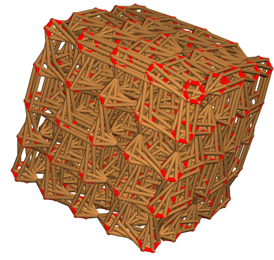
The red hexagons here are just visual guides; the true object simply has connections that knit together the “group elements” on each fiber. And the remarkable thing is that this can be thought of as a very direct discrete approximation to a fiber bundle—where the connections correspond quite literally to the so-called connections in the fiber bundle, that “align” the copies of the gauge group at each point, and in effect implement the covariant derivative.
In our models the structure of the discrete analog of the fiber bundle has to emerge from the actual operation of underlying hypergraph rules. And most likely this happens because there are multiple ways in which a given rule can locally be applied to a hypergraph, effectively leading to the kind of local symmetry we see appearing at every point of the base space.
But even without knowing any of the details of this, we can already work some things out just from the structure of our “fiber bundle graph”. For example, consider tracing out “Wilson loops” which visit fibers around a closed loop—and ask what the “total group action” associated with this process is. But by direct analogy with electromagnetism we can now interpret this as the “magnetic flux through the Wilson loop”.
But what happens if we look at the total flux emanating from a closed volume? For topological reasons, it’s inevitable that this is quantized. And even in the simple setup shown here we can start to interpret nonzero values as corresponding to the presence of “magnetic monopoles”.
Not Even Just Fundamental Physics
I developed what are now being called “Wolfram models” to be as a minimal and general as possible. And—perhaps not too surprisingly therefore—the models are looking as if they’re also very relevant for all sorts of things beyond fundamental physics. Several of these things got studied at the Summer School, notably in mathematics, in biology and in other areas of physics.
The applications in mathematics look to be particularly deep, and we’ve actually been working quite intensively on them over the past couple of weeks—leading to some rather exciting conclusions that I’m hoping to write about soon.
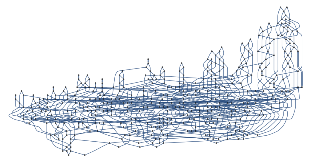
When it comes to biology, it seems possible that our models may be able to provide a new approach to thinking about biological evolution, and at the Summer School Antonia Kaestner and Tali Beynon started trying to understand how graphs—and multiway systems—might be used to represent evolutionary processes:
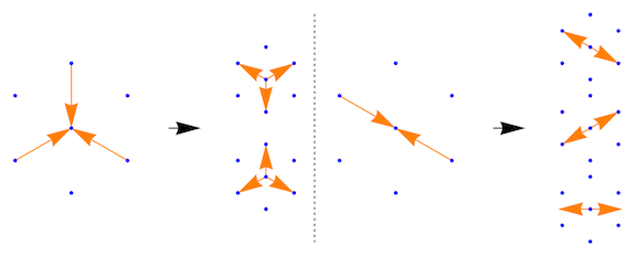
Another project at the Summer School, by Matthew Kafker (working with Christopher Wolfram), concerned hard sphere gases. I have a long personal history with hard sphere gases: looking at them was what first got me interested—back in 1972—in questions about the emergence of complexity. So I was quite surprised that after all these years, there was something new to consider with them. But a feature of our models is that they suggest a different way to look at systems.
So what if we think of the collisions in a hard sphere gas as events? Then—just like in our models—we can make a causal graph that shows the causal relationships between these events:
And—just like in our models—we can define light cones and so on. But what does this tell us about hard sphere gases? Standard statistical mechanics approaches look at local statistical properties—in a sense making a “molecular chaos” assumption that everything else is random. But the causal graph has the potential to give us much more global (and long-range) information—which is likely to be increasingly important as the density of the hard sphere gas increases.
Hard sphere gases are based on classical physics. But given that our models naturally include quantum mechanics, does that give us a way to study quantum gases, or quantum fluids? At the Summer School Ivan Martinez studied a quantum generalization of my 1986 cellular automaton fluids model.
In that model discrete idealized molecules undergo 2- and 3-body collisions. And when I originally set this up, I just picked possible outcomes from these collisions consistent with momentum conservation. But there are several choices to make—and with the understanding we now have, the obvious thing to do is just to follow all choices, and make a multiway system. Here are the collisions and possible outcomes:
A single branch of the multiway system produces a specific pattern of fluid flow. But the whole multiway system represents a whole collection of quantum states—or in effect a quantum fluid (and in the most obvious version of the model, a Fermi fluid). So now we can start to ask questions about the quantum fluid, studying branchial graphs, event horizons, etc.
And Lots of Other Projects Too…

I’ve talked about 11 projects so far here—but that’s less than a third of all the Wolfram Physics–related projects at the Summer School.
There were projects about the large-scale structure of hypergraphs, and phenomena like the spatial distribution of dimension, time variation of dimension and possible overall growth rates of hypergraphs. There was a project about characterizing overall structures of hypergraphs by finding PDE modes on them (“Weyl’s law for graphs”).
What happens if you look at the space of all possible hypergraphs, and for example form state transition graphs by applying rules? One project explored subgraphs excluded by evolution (“the approach to attractor states”). Another project explored the structure of the space of possible hypergraphs, and the mathematical analysis of ergodicity in it.
One of the upcoming challenges in our models is about identifying “particles” and their properties. One project started directly hunting for particles by looking at the effects of perturbations in hypergraphs. Another studied the dynamics of specific kinds of “topologically stable defects” in hypergraphs. There was a project looking for global conservation laws in hypergraph rewriting, and another studying local graph invariants. There was also a project that started to make a rather direct detector of gravitational waves in our models.
There were projects that analysed the global behavior of our models. One continued the enumeration of cases in which black holes arise. Another looked at termination and completion in multiway systems. Still another compared growth in physical vs. branchial space.
I mentioned above the concept of “proof by compilation” and its use in validating the quantum features of our models. One project at the Summer School began the process of using our models as a foundation for practical “numerical general relativity” (in much the same way as my cellular automata fluids have become the basis for practical fluid computations).
There are lots of interesting questions about how our models relate to known features of physics. And there were projects at the Summer School about understanding the emergence of rotational invariance and CPT invariance as well as the AdS/CFT correspondence (and things like the Bekenstein bound).
There were projects about the Wolfram Physics Project not only at our Summer School, but also at our High School Summer Camp. One explored the emergent differential geometry of a particular one of our models that makes something like a manifold with curvature. Others explored fundamental aspects of models like ours. One searched for multiway systems with intermediate growth. Another explored multiway systems based on cyclic string substitutions.
There were still other projects at both the Summer School and Summer Camp that explored systems from the computational universe—now informed by ideas from the Wolfram Physics Project. One looked at non-deterministic Turing machines; another looked at combinators.
I suggested most of the projects I’ve discussed here, and that makes it particularly satisfying for me to see how well they’ve progressed. Few are yet “finished”, but they’re all off and running, beginning to build up a serious corpus of work around the Wolfram Physics Project. And I’m looking forward to seeing how they develop, what they discover, how they turn into papers—and how they seed other work which will help explore the amazing basic science opportunity that’s opened up with the Wolfram Physics Project.