An Unexpected Correspondence
Enter any expression and it’ll get evaluated:
And internally—say in the Wolfram Language—what’s going on is that the expression is progressively being transformed using all available rules until no more rules apply. Here the process can be represented like this:

We can think of the yellow boxes in this picture as corresponding to “evaluation events” that transform one “state of the expression” (represented by a blue box) to another, eventually reaching the “fixed point” 12.
And so far this may all seem very simple. But actually there are many surprisingly complicated and deep issues and questions. For example, to what extent can the evaluation events be applied in different orders, or in parallel? Does one always get the same answer? What about non-terminating sequences of events? And so on.
I was first exposed to such issues more than 40 years ago—when I was working on the design of the evaluator for the SMP system that was the forerunner of Mathematica and the Wolfram Language. And back then I came up with pragmatic, practical solutions—many of which we still use today. But I was never satisfied with the whole conceptual framework. And I always thought that there should be a much more principled way to think about such things—that would likely lead to all sorts of important generalizations and optimizations.
Well, more than 40 years later I think we can finally now see how to do this. And it’s all based on ideas from our Physics Project—and on a fundamental correspondence between what’s happening at the lowest level in all physical processes and in expression evaluation. Our Physics Project implies that ultimately the universe evolves through a series of discrete events that transform the underlying structure of the universe (say, represented as a hypergraph)—just like evaluation events transform the underlying structure of an expression.
And given this correspondence, we can start applying ideas from physics—like ones about spacetime and quantum mechanics—to questions of expression evaluation. Some of what this will lead us to is deeply abstract. But some of it has immediate practical implications, notably for parallel, distributed, nondeterministic and quantum-style computing. And from seeing how things play out in the rather accessible and concrete area of expression evaluation, we’ll be able to develop more intuition about fundamental physics and about other areas (like metamathematics) where the ideas of our Physics Project can be applied.
Causal Graphs and Spacetime
The standard evaluator in the Wolfram Language applies evaluation events to an expression in a particular order. But typically multiple orders are possible; for the example above, there are three:

So what determines what orders are possible? There is ultimately just one constraint: the causal dependencies that exist between events. The key point is that a given event cannot happen unless all the inputs to it are available, i.e. have already been computed. So in the example here, the ![]() evaluation event cannot occur unless the
evaluation event cannot occur unless the ![]() one has already occurred. And we can summarize this by “drawing a causal edge” from the
one has already occurred. And we can summarize this by “drawing a causal edge” from the ![]() event to the
event to the ![]() one. Putting together all these “causal relations”, we can make a causal graph, which in the example here has the simple form (where we include a special “Big Bang” initial event to create the original expression that we’re evaluating):
one. Putting together all these “causal relations”, we can make a causal graph, which in the example here has the simple form (where we include a special “Big Bang” initial event to create the original expression that we’re evaluating):

What we see from this causal graph is that the events on the left must all follow each other, while the event on the right can happen “independently”. And this is where we can start making an analogy with physics. Imagine our events are laid out in spacetime. The events on the left are “timelike separated” from each other, because they are constrained to follow one after another, and so must in effect “happen at different times”. But what about the event on the right? We can think of this as being “spacelike separated” from the others, and happening at a “different place in space” asynchronously from the others.
As a quintessential example of a timelike chain of events, consider making the definition
and then generating the causal graph for the events associated with evaluating f[f[f[1]]] (i.e. Nest[f, 1, 3]):

A straightforward way to get spacelike events is just to “build in space” by giving an expression like f[1] + f[1] + f[1] that has parts that can effectively be thought of as being explicitly “laid out in different places”, like the cells in a cellular automaton:

But one of the major lessons of our Physics Project is that it’s possible for space to “emerge dynamically” from the evolution of a system (in that case, by successive rewriting of hypergraphs). And it turns out very much the same kind of thing can happen in expression evaluation, notably with recursively defined functions.
As a simple example, consider the standard definition of Fibonacci numbers:
With this definition, the causal graph for the evaluation of f[3] is then:

For f[5], dropping the “context” of each event, and showing only what changed, the graph is

while for f[8] the structure of the graph is:

So what is the significance of there being spacelike-separated parts in this graph? At a practical level, a consequence is that those parts correspond to subevaluations that can be done independently, for example in parallel. All the events (or subevaluations) in any timelike chain must be done in sequence. But spacelike-separated events (or subevaluations) don’t immediately have a particular relative order. The whole graph can be thought of as defining a partial ordering for all events—with the events forming a partially ordered set (poset). Our “timelike chains” then correspond to what are usually called chains in the poset. The antichains of the poset represent possible collections of events that can occur “simultaneously”.
And now there’s a deep analogy to physics. Because just like in the standard relativistic approach to spacetime, we can define a sequence of “spacelike surfaces” (or hypersurfaces in 3 + 1-dimensional spacetime) that correspond to possible successive “simultaneity surfaces” where events can consistently be done simultaneously. Put another way, any “foliation” of the causal graph defines a sequence of “time steps” in which particular collections of events occur—as in for example:

And just like in relativity theory, different foliations correspond to different choices of reference frames, or what amount to different choices of “space and time coordinates”. But at least in the examples we’ve seen so far, the “final result” from the evaluation is always the same, regardless of the foliation (or reference frame) we use—just as we expect when there is relativistic invariance.
As a slightly more complex—but ultimately very similar—example, consider the nestedly recursive function:
Now the causal graph for f[12] has the form

which again has both spacelike and timelike structure.
Foliations and the Definition of Time
Let’s go back to our first example above—the evaluation of (1 + (2 + 2)) + (3 + 4). As we saw above, the causal graph in this case is:

The standard Wolfram Language evaluator makes these events occur in the following order:

And by applying events in this order starting with the initial state, we can reconstruct the sequence of states that will be reached at each step by this particular evaluation process (where now we’ve highlighted in each state the part that’s going to be transformed at each step):

Here’s the standard evaluation order for the Fibonacci number f[3]:

And here’s the sequence of states generated from this sequence of events:

Any valid evaluation order has to eventually visit (i.e. apply) all the events in the causal graph. Here’s the path that’s traced out by the standard evaluation order on the causal graph for f[8]. As we’ll discuss later, this corresponds to a depth-first scan of the (directed) graph:

But let’s return now to our first example. We’ve seen the order of events used in the standard Wolfram Language evaluation process. But there are actually three different orders that are consistent with the causal relations defined by the causal graph (in the language of posets, each of these is a “total ordering”):

And for each of these orders we can reconstruct the sequence of states that would be generated:

Up to this point we’ve always assumed that we’re just applying one event at a time. But whenever we have spacelike-separated events, we can treat such events as “simultaneous”—and applied at the same point. And—just like in relativity theory—there are typically multiple possible choices of “simultaneity surfaces”. Each one corresponds to a certain foliation of our causal graph. And in the simple case we’re looking at here, there are only two possible (maximal) foliations:

From such foliations we can reconstruct possible total orderings of individual events just by enumerating possible permutations of events within each slice of the foliation (i.e. within each simultaneity surface). But we only really need a total ordering of events if we’re going to apply one event at a time. Yet the whole point is that we can view spacelike-separated events as being “simultaneous”. Or, in other words, we can view our system as “evolving in time”, with each “time step” corresponding to a successive slice in the foliation.
And with this setup, we can reconstruct states that exist at each time step—interspersed by updates that may involve several “simultaneous” (spacelike-separated) events. In the case of the two foliations above, the resulting sequences of (“reconstructed”) states and updates are respectively:

As a more complicated example, consider recursively evaluating the Fibonacci number f[3] as above. Now the possible (maximal) foliations are:

For each of these foliations we can then reconstruct an explicit “time series” of states, interspersed by “updates” involving varying numbers of events:

So where in all these is the standard evaluation order? Well, it’s not explicitly here—because it involves doing a single event at a time, while all the foliations here are “maximal” in the sense that they aggregate as many events as they can into each spacelike slice. But if we don’t impose this maximality constraint, are there foliations that in a sense “cover” the standard evaluation order? Without the maximality constraint, there turn out in the example we’re using to be not 10 but 1249 possible foliations. And there are 4 that “cover” the standard (“depth-first”) evaluation order (indicated by a dashed red line):

(Only the last foliation here, in which every “slice” is just a single event, can strictly reproduce the standard evaluation order, but the others are all still “consistent with it”.)
In the standard evaluation process, only a single event is ever done at a time. But what if instead one tries to do as many events as possible at a time? Well, that’s what our “maximal foliations” above are about. But one particularly notable case is what corresponds to a breadth-first scan of the causal graph. And this turns out to be covered by the very last maximal foliation we showed above.
How this works may not be immediately obvious from the picture. With our standard layout for the causal graph, the path corresponding to the breadth-first scan is:

But if we lay out the causal graph differently, the path takes on the much-more-obviously-breadth-first form:

And now using this layout for the various configurations of foliations above we get:

We can think of different layouts for the causal graph as defining different “coordinatizations of spacetime”. If the vertical direction is taken to be time, and the horizontal direction space, then different layouts in effect place events at different positions in time and space. And with the layout here, the last foliation above is “flat”, in the sense that successive slices of the foliation can be thought of as directly corresponding to successive “steps in time”.
In physics terms, different foliations correspond to different “reference frames”. And the “flat” foliation can be thought of as being like the cosmological rest frame, in which the observer is “at rest with respect to the universe”. In terms of states and events, we can also interpret this another way: we can say it’s the foliation in which in some sense the “largest possible number of events are being packed in at each step”. Or, more precisely, if at each step we scan from left to right, we’re doing every successive event that doesn’t overlap with events we’ve already done at this step:

And actually this also corresponds to what happens if, instead of using the built-in standard evaluator, we explicitly tell the Wolfram Language to repeatedly do replacements in expressions. To compare with what we’ve done above, we have to be a little careful in our definitions, using ⊕ and ⊖ as versions of + and – that have to get explicitly evaluated by other rules. But having done this, we get exactly the same sequence of “intermediate expressions” as in the flat (i.e. “breadth-first”) foliation above:

In general, different foliations can be thought of as specifying different “event-selection functions” to be applied to determine what events should occur at the next steps from any given state. At one extreme we can pick single-event-at-a-time event selection functions—and at the other extreme we can pick maximum-events-at-a-time event selection functions. In our Physics Project we have called the states obtained by applying maximal collections of events at a time “generational states”. And in effect these states represent the typical way we parse physical “spacetime”—in which we take in “all of space” at every successive moment of time. At a practical level the reason we do this is that the speed of light is somehow fast compared to the operation of our brains: if we look at our local surroundings (say the few hundred meters around us), light from these will reach us in a microsecond, while it takes our brains milliseconds to register what we’re seeing. And this makes it reasonable for us to think of there being an “instantaneous state of space” that we can perceive “all at once” at each particular “moment in time”.
But what’s the analog of this when it comes to expression evaluation? We’ll discuss this a little more later. But suffice it to say here that it depends on who or what the “observer” of the process of evaluation is supposed to be. If we’ve got different elements of our states laid out explicitly in arrays, say in a GPU, then we might again “perceive all of space at once”. But if, for example, the data associated with states is connected through chains of pointers in memory or the like, and we “observe” this data only when we explicitly follow these pointers, then our perception won’t as obviously involve something we can think of as “bulk space”. But by thinking in terms of foliations (or reference frames) as we have here, we can potentially fit what’s going on into something like space, that seems familiar to us. Or, put another way, we can imagine in effect “programming in a certain reference frame” in which we can aggregate multiple elements of what’s going on into something we can consider as an analog of space—thereby making it familiar enough for us to understand and reason about.
Multiway Evaluation and Multiway Graphs
We can view everything we’ve done so far as dissecting and reorganizing the standard evaluation process. But let’s say we’re just given certain underlying rules for transforming expressions—and then we apply them in all possible ways. It’ll give us a “multiway” generalization of evaluation—in which instead of there being just one path of history, there are many. And in our Physics Project, this is exactly how the transition from classical to quantum physics works. And as we proceed here, we’ll see a close correspondence between multiway evaluation and quantum processes.
But let’s start again with our expression (1 + (2 + 2)) + (3 + 4), and consider all possible ways that individual integer addition “events” can be applied to evaluate this expression. In this particular case, the result is pretty simple, and can be represented by a tree that branches in just two places:

But one thing to notice here is that even at the first step there’s an event ![]() that we’ve never seen before. It’s something that’s possible if we apply integer addition in all possible places. But when we start from the standard evaluation process, the basic event
that we’ve never seen before. It’s something that’s possible if we apply integer addition in all possible places. But when we start from the standard evaluation process, the basic event ![]() just never appears with the “expression context” we’re seeing it in here.
just never appears with the “expression context” we’re seeing it in here.
Each branch in the tree above in some sense represents a different “path of history”. But there’s a certain redundancy in having all these separate paths—because there are multiple instances of the same expression that appear in different places. And if we treat these as equivalent and merge them we now get:

(The question of “state equivalence” is a subtle one, that ultimately depends on the operation of the observer, and how the observer constructs their perception of what’s going on. But for our purposes here, we’ll treat expressions as equivalent if they are structurally the same, i.e. every instance of ![]() or of 5 is “the same”
or of 5 is “the same” ![]() or 5.)
or 5.)
If we now look only at states (i.e. expressions) we’ll get a multiway graph, of the kind that’s appeared in our Physics Project and in many applications of concepts from it:

This graph in a sense gives a succinct summary of possible paths of history, which here correspond to possible evaluation paths. The standard evaluation process corresponds to a particular path in this multiway graph:

What about a more complicated case? For example, what is the multiway graph for our recursive computation of Fibonacci numbers? As we’ll discuss at more length below, in order to make sure every branch of our recursive evaluation terminates, we have to give a slightly more careful definition of our function f:
But now here’s the multiway tree for the evaluation of f[2]:

And here’s the corresponding multiway graph:

The leftmost branch in the multiway tree corresponds to the standard evaluation process; here’s the corresponding path in the multiway graph:

Here’s the structure of the multiway graph for the evaluation of f[3]:

Note that (as we’ll discuss more later) all the possible evaluation paths in this case lead to the same final expression, and in fact in this particular example all the paths are of the same length (12 steps, i.e. 12 evaluation events).
In the multiway graphs we’re drawing here, every edge in effect corresponds to an evaluation event. And we can imagine setting up foliations in the multiway graph that divide these events into slices. But what is the significance of these slices? When we did the same kind of thing above for causal graphs, we could interpret the slices as representing “instantaneous states laid out in space”. And by analogy we can interpret a slice in the multiway graph as representing “instantaneous states laid out across branches of history”. In the context of our Physics Project, we can then think of these slices as being like superpositions in quantum mechanics, or states “laid out in branchial space”. And, as we’ll discuss later, just as we can think of elements laid out in “space” as corresponding in the Wolfram Language to parts in a symbolic expression (like a list, a sum, etc.), so now we’re dealing with a new kind of way of aggregating states across branchial space, that has to be represented with new language constructs.
But let’s return to the very simple case of (1 + (2 + 2)) + (3 + 4). Here’s a more complete representation of the multiway evaluation process in this case, including both all the events involved, and the causal relations between them:

The “single-way” evaluation process we discussed above uses only part of this:

And from this part we can pull out the causal relations between events to reproduce the (“single-way”) causal graph we had before. But what if we pull out all the causal relations in our full graph?

What we then have is the multiway causal graph. And from foliations of this, we can construct possible histories—though now they’re multiway histories, with the states at particular time steps now being what amount to superposition states.
In the particular case we’re showing here, the multiway causal graph has a very simple structure, consisting essentially just of a bunch of isomorphic pieces. And as we’ll see later, this is an inevitable consequence of the nature of the evaluation we’re doing here, and its property of causal invariance (and in this case, confluence).
Branchlike Separation
Although what we’ve discussed has already been somewhat complicated, there’s actually been a crucial simplifying assumption in everything we’ve done. We’ve assumed that different transformations on a given expression can never apply to the same part of the expression. Different transformations can apply to different parts of the same expression (corresponding to spacelike-separated evaluation events). But there’s never been a “conflict” between transformations, where multiple transformations can apply to the same part of the same expression.
So what happens if we relax this assumption? In effect it means that we can generate different “incompatible” branches of history—and we can characterize the events that produce this as “branchlike separated”. And when such branchlike-separated events are applied to a given state, they’ll produce multiple states which we can characterize as “separated in branchial space”, but nevertheless correlated as a result of their “common ancestry”—or, in quantum mechanics terms, “entangled”.
As a very simple first example, consider the rather trivial function f defined by
If we evaluate f[f[0]] (for any f) there are immediately two “conflicting” branches: one associated with evaluation of the “outer f”, and one with evaluation of the “inner f”:

We can indicate branchlike-separated pairs of events by a dashed line:

Adding in causal edges, and merging equivalent states, we get:

We see that some events are causally related. The first two events are not—but given that they involve overlapping transformations they are “branchially related” (or, in effect, entangled).
Evaluating the expression f[f[0]+1] gives a more complicated graph, with two different instances of branchlike-separated events:

Extracting the multiway states graph we get

where now we have indicated “branchially connected” states by pink “branchial edges”. Pulling out only these branchial edges then gives the (rather trivial) branchial graph for this evaluation process:

There are many subtle things going on here, particularly related to the treelike structure of expressions. We’ve talked about separations between events: timelike, spacelike and branchlike. But what about separations between elements of an expression? In something like {f[0], f[0], f[0]} it’s reasonable to extend our characterization of separations between events, and say that the f[0]’s in the expression can themselves be considered spacelike separated. But what about in something like f[f[0]]? We can say that the f[_]’s here “overlap”—and “conflict” when they are transformed—making them branchlike separated. But the structure of the expression also inevitably makes them “treelike separated”. We’ll see later how to think about the relation between treelike-separated elements in more fundamental terms, ultimately using hypergraphs. But for now an obvious question is what in general the relation between branchlike-separated elements can be.
And essentially the answer is that branchlike separation has to “come with” some other form of separation: spacelike, treelike, rulelike, etc. Rulelike separation involves having multiple rules for the same object (e.g. a rule ![]() as well as
as well as ![]() )—and we’ll talk about this later. With spacelike separation, we basically get branchlike separation when subexpressions “overlap”. This is fairly subtle for tree-structured expressions, but is much more straightforward for strings, and indeed we have discussed this case extensively in connection with our Physics Project.
)—and we’ll talk about this later. With spacelike separation, we basically get branchlike separation when subexpressions “overlap”. This is fairly subtle for tree-structured expressions, but is much more straightforward for strings, and indeed we have discussed this case extensively in connection with our Physics Project.
Consider the (rather trivial) string rewriting rule:
Applying this rule to AAAAAA we get:

Some of the events here are purely spacelike separated, but whenever the characters they involve overlap, they are also branchlike separated (as indicated by the dashed pink lines). Extracting the multiway states graph we get:

And now we get the following branchial graph:

So how can we see analogs in expression evaluation? It turns out that combinators provide a good example (and, yes, it’s quite remarkable that we’re using combinators here to help explain something—given that combinators almost always seem like the most obscure and difficult-to-explain things around). Define the standard S and K combinators:
Now we have for example

where there are many spacelike-separated events, and a single pair of branchlike + treelike-separated ones. With a slightly more complicated initial expression, we get the rather messy result

now with many branchlike-separated states:

Rather than using the full standard S, K combinators, we can consider a simpler combinator definition:
Now we have for example

where the branchial graph is

and the multiway causal graph is:

The expression f[f[f][f]][f] gives a more complicated multiway graph

and branchial graph:

Interpretations, Analogies and the Concept of Multi
Before we started talking about branchlike separation, the only kinds of separation we considered were timelike and spacelike. And in this case we were able to take the causal graphs we got, and set up foliations of them where each slice could be thought of as representing a sequential step in time. In effect, what we were doing was to aggregate things so that we could talk about what happens in “all of space” at a particular time.
But when there’s branchlike separation we can no longer do this. Because now there isn’t a single, consistent “configuration of all of space” that can be thought of as evolving in a single thread through time. Rather, there are “multiple threads of history” that wind their way through the branchings (and mergings) that occur in the multiway graph. One can make foliations in the multiway graph—much like one does in the causal graph. (More strictly, one really needs to make the foliations in the multiway causal graph—but these can be “inherited” by the multiway graph.)
In physics terms, the (single-way) causal graph can be thought of as a discrete version of ordinary spacetime—with a foliation of it specifying a “reference frame” that leads to a particular identification of what one considers space, and what time. But what about the multiway causal graph? In effect, we can imagine that it defines a new, branchial “direction”, in addition to the spatial direction. Projecting in this branchial direction, we can then think of getting a kind of branchial analog of spacetime that we can call branchtime. And when we construct the multiway graph, we can basically imagine that it’s a representation of branchtime.
A particular slice of a foliation of the (single-way) causal graph can be thought of as corresponding to an “instantaneous state of (ordinary) space”. So what does a slice in a foliation of the multiway graph represent? It’s effectively a branchial or multiway combination of states—a collection of states that can somehow all exist “at the same time”. And in physics terms we can interpret it as a quantum superposition of states.
But how does all this work in the context of expressions? The parts of a single expression like
In ordinary evaluation, we just generate a specific sequence of individual expressions. But in multiway evaluation, we can imagine that we generate a sequence of Multi objects. In the examples we’ve seen so far, we always eventually get a Multi containing just a single expression. But we’ll soon find out that that’s not always how things work, and we can perfectly well end up with a Multi containing multiple expressions.
So what might we do with a Multi? In a typical “nondeterministic computation” we probably want to ask: “Does the Multi contain some particular expression or pattern that we’re looking for?” If we imagine that we’re doing a “probabilistic computation” we might want to ask about the frequencies of different kinds of expressions in the Multi. And if we’re doing quantum computation with the normal formalism of quantum mechanics, we might want to tag the elements of the Multi with “quantum amplitudes” (that, yes, in our model presumably have magnitudes determined by path counting in the multiway graph, and phases representing the “positions of elements in branchial space”). And in a traditional quantum measurement, the concept would typically be to determine a projection of a Multi, or in effect an inner product of Multi objects. (And, yes, if one knows only that projection, it’s not going to be enough to let one unambiguously continue the “multiway computation”; the quantum state has in effect been “collapsed”.)
Is There Always a Definite Result?
For an expression like (1 + (2 + 2)) + (3 + 4) it doesn’t matter in what order one evaluates things; one always gets the same result—so that the corresponding multiway graph leads to just a single final state:

But it’s not always true that there’s a single final state. For example, with the definitions
standard evaluation in the Wolfram Language gives the result 0 for f[f[0]] but the full multiway graph shows that (with a different evaluation order) it’s possible instead to get the result g[g[0]]:

And in general when a certain collection of rules (or definitions) always leads to just a single result, one says that the collection of rules is confluent; otherwise it’s not. Pure arithmetic turns out to be confluent. But there are plenty of examples (e.g. in string rewriting) that are not. Ultimately a failure of confluence must come from the presence of branchlike separation—or in effect a conflict between behavior on two different branches. And so in the example above we see that there are branchlike-separated “conflicting” events that never resolve—yielding two different final outcomes:

As an even simpler example, consider the definitions ![]() and
and ![]() . In the Wolfram Language these definitions immediately overwrite each other. But assume they could both be applied (say through explicit
. In the Wolfram Language these definitions immediately overwrite each other. But assume they could both be applied (say through explicit ![]() ,
, ![]() rules). Then there’s a multiway graph with two “unresolved” branches—and two outcomes:
rules). Then there’s a multiway graph with two “unresolved” branches—and two outcomes:

For string rewriting systems, it’s easy to enumerate possible rules. The rule
(that effectively sorts the elements in the string) is confluent:

But the rule
is not confluent

and “evaluates” BABABA to four distinct outcomes:
These are all cases where “internal conflicts” lead to multiple different final results. But another way to get different results is through “side effects”. Consider first setting x = 0 then evaluating {x = 1, x + 1}:

If the order of evaluation is such that x + 1 is evaluated before x = 1 it will give 1, otherwise it will give 2, leading to the two different outcomes {1, 1} and {1, 2}. In some ways this is like the example above where we had two distinct rules: ![]() and
and ![]() . But there’s a difference. While explicit rules are essentially applied only “instantaneously”, an assignment like x = 1 has a “permanent” effect, at least until it is “overwritten” by another assignment. In an evaluation graph like the one above we’re showing particular expressions generated during the evaluation process. But when there are assignments, there’s an additional “hidden state” that in the Wolfram Language one can think of as corresponding to the state of the global symbol table. If we included this, then we’d again see rules that apply “instantaneously”, and we’d be able to explicitly trace causal dependencies between events. But if we elide it, then we effectively hide the causal dependence that’s “carried” by the state of the symbol table, and the evaluation graphs we’ve been drawing are necessarily somewhat incomplete.
. But there’s a difference. While explicit rules are essentially applied only “instantaneously”, an assignment like x = 1 has a “permanent” effect, at least until it is “overwritten” by another assignment. In an evaluation graph like the one above we’re showing particular expressions generated during the evaluation process. But when there are assignments, there’s an additional “hidden state” that in the Wolfram Language one can think of as corresponding to the state of the global symbol table. If we included this, then we’d again see rules that apply “instantaneously”, and we’d be able to explicitly trace causal dependencies between events. But if we elide it, then we effectively hide the causal dependence that’s “carried” by the state of the symbol table, and the evaluation graphs we’ve been drawing are necessarily somewhat incomplete.
Computations That Never End
The basic operation of the Wolfram Language evaluator is to keep doing transformations until the result no longer changes (or, in other words, until a fixed point is reached). And that’s convenient for being able to “get a definite answer”. But it’s rather different from what one usually imagines happens in physics. Because in that case we’re typically dealing with things that just “keep progressing through time”, without ever getting to any fixed point. (“Spacetime singularities”, say in black holes, do for example involve reaching fixed points where “time has come to an end”.)
But what happens in the Wolfram Language if we just type ![]() , without giving any value to
, without giving any value to ![]() ? The Wolfram Language evaluator will keep evaluating this, trying to reach a fixed point. But it’ll never get there. And in practice it’ll give a message, and (at least in Version 13.3 and above) return a TerminatedEvaluation object:
? The Wolfram Language evaluator will keep evaluating this, trying to reach a fixed point. But it’ll never get there. And in practice it’ll give a message, and (at least in Version 13.3 and above) return a TerminatedEvaluation object:

What’s going on inside here? If we look at the evaluation graph, we can see that it involves an infinite chain of evaluation events, that progressively “extrude” +1’s:

A slightly simpler case (that doesn’t raise questions about the evaluation of Plus) is to consider the definition
which has the effect of generating an infinite chain of progressively more “f-nested” expressions:

Let’s say we define two functions:
Now we don’t just get a simple chain of results; instead we get an exponentially growing multiway graph:

In general, whenever we have a recursive definition (say of f in terms of f or x in terms of x) there’s the possibility of an infinite process of evaluation, with no “final fixed point”. There are of course specific cases of recursive definitions that always terminate—like the Fibonacci example we gave above. And indeed when we’re dealing with so-called “primitive recursion” this is how things inevitably work: we’re always “systematically counting down” to some defined base case (say
When we look at string rewriting (or, for that matter, hypergraph rewriting), evolution that doesn’t terminate is quite ubiquitous. And in direct analogy with, for example, the string rewriting rule A![]() BBB, BB
BBB, BB![]() A we can set up the definitions
A we can set up the definitions
and then the (infinite) multiway graph begins:

One might think that the possibility of evaluation processes that don’t terminate would be a fundamental problem for a system set up like the Wolfram Language. But it turns out that in current normal usage one basically never runs into the issue except by mistake, when there’s a bug in one’s program.
Still, if one explicitly wants to generate an infinite evaluation structure, it’s not hard to do so. Beyond ![]() one can define
one can define
and then one gets the multiway graph

which has CatalanNumber[t] (or asymptotically ~4t) states at layer t.
Another “common bug” form of non-terminating evaluation arises when one makes a primitive-recursion-style definition without giving a “boundary condition”. Here, for example, is the Fibonacci recursion without f[0] and f[1] defined:
And in this case the multiway graph is infinite

with ~2t states at layer t.
But consider now the “unterminated factorial recursion”
On its own, this just leads to a single infinite chain of evaluation

but if we add the explicit rule that multiplying anything by zero gives zero (i.e. 0 _ → 0) then we get

in which there’s a “zero sink” in addition to an infinite chain of f[–n] evaluations.
Some definitions have the property that they provably always terminate, though it may take a while. An example is the combinator definition we made above:
Here’s the multiway graph starting with f[f[f][f]][f], and terminating in at most 10 steps:

Starting with f[f[f][f][f][f]][f] the multiway graph becomes

but again the evaluation always terminates (and gives a unique result). In this case we can see why this happens: at each step f[x_][y_] effectively “discards ![]() ”, thereby “fundamentally getting smaller”, even as it “puffs up” by making three copies of
”, thereby “fundamentally getting smaller”, even as it “puffs up” by making three copies of ![]() .
.
But if instead one uses the definition
things get more complicated. In some cases, the multiway evaluation always terminates

while in others, it never terminates:

But then there are cases where there is sometimes termination, and sometimes not:

In this particular case, what’s happening is that evaluation of the first argument of the “top-level f” never terminates, but if the top-level f is evaluated before its arguments then there’s immediate termination. Since the standard Wolfram Language evaluator evaluates arguments first (“leftmost-innermost evaluation”), it therefore won’t terminate in this case—even though there are branches in the multiway evaluation (corresponding to “outermost evaluation”) that do terminate.
Transfinite Evaluation
If a computation reaches a fixed point, we can reasonably say that that’s the “result” of the computation. But what if the computation goes on forever? Might there still be some “symbolic” way to represent what happens—that for example allows one to compare results from different infinite computations?
In the case of ordinary numbers, we know that we can define a “symbolic infinity” ∞ (Infinity in Wolfram Language) that represents an infinite number and has all the obvious basic arithmetic properties:
But what about infinite processes, or, more specifically, infinite multiway graphs? Is there some useful symbolic way to represent such things? Yes, they’re all “infinite”. But somehow we’d like to distinguish between infinite graphs of different forms, say:
And already for integers, it’s been known for more than a century that there’s a more detailed way to characterize infinities than just referring to them all as ∞: it’s to use the idea of transfinite numbers. And in our case we can imagine successively numbering the nodes in a multiway graph, and seeing what the largest number we reach is. For an infinite graph of the form
(obtained say from x = x + 1 or x = {x}) we can label the nodes with successive integers, and we can say that the “largest number reached” is the transfinite ordinal ω.
A graph consisting of two infinite chains is then characterized by 2ω, while an infinite 2D grid is characterized by ω2, and an infinite binary tree is characterized by 2ω.
What about larger numbers? To get to ωω we can use a rule like
that effectively yields a multiway graph that corresponds to a tree in which successive layers have progressively larger numbers of branches:
One can think of a definition like x = x + 1 as setting up a “self-referential data structure”, whose specification is finite (in this case essentially a loop), and where the infinite evaluation process arises only when one tries to get an explicit value out of the structure. More elaborate recursive definitions can’t, however, readily be thought of as setting up straightforward self-referential data structures. But they still seem able to be characterized by transfinite numbers.
In general many multiway graphs that differ in detail will be associated with a given transfinite number. But the expectation is that transfinite numbers can potentially provide robust characterizations of infinite evaluation processes, with different constructions of the “same evaluation” able to be identified as being associated with the same canonical transfinite number.
Most likely, definitions purely involving pattern matching won’t be able to generate infinite evaluations beyond ε0 = ωωω...—which is also the limit of where one can reach with proofs based on ordinary induction, Peano Arithmetic, etc. It’s perfectly possible to go further—but one needs to explicitly use functions like NestWhile etc. in the definitions that are given.
And there’s another issue as well: given a particular set of definitions, there’s no limit to how difficult it can be to determine the ultimate multiway graph that’ll be produced. In the end this is a consequence of computational irreducibility, and of the undecidability of the halting problem, etc. And what one can expect in the end is that some infinite evaluation processes one will be able to prove can be characterized by particular transfinite numbers, but others one won’t be able to “tie down” in this way—and in general, as computational irreducibility might suggest, won’t ever allow one to give a “finite symbolic summary”.
The Question of the Observer
One of the key lessons of our Physics Project is the importance of the character of the observer in determining what one “takes away” from a given underlying system. And in setting up the evaluation process—say in the Wolfram Language—the typical objective is to align with the way human observers expect to operate. And so, for example, one normally expects that one will give an expression as input, then in the end get an expression as output. The process of transforming input to output is analogous to the doing of a calculation, the answering of a question, the making of a decision, the forming of a response in human dialog, and potentially the forming of a thought in our minds. In all of these cases, we treat there as being a certain “static” output.
It’s very different from the way physics operates, because in physics “time always goes on”: there’s (essentially) always another step of computation to be done. In our usual description of evaluation, we talk about “reaching a fixed point”. But an alternative would be to say that we reach a state that just repeats unchanged forever—but we as observers equivalence all those repeats, and think of it as having reached a single, unchanging state.
Any modern practical computer also fundamentally works much more like physics: there are always computational operations going on—even though those operations may end up, say, continually putting the exact same pixel in the same place on the screen, so that we can “summarize” what’s going on by saying that we’ve reached a fixed point.
There’s much that can be done with computations that reach fixed points, or, equivalently with functions that return definite values. And in particular it’s straightforward to compose such computations or functions, continually taking output and then feeding it in as input. But there’s a whole world of other possibilities that open up once one can deal with infinite computations. As a practical matter, one can treat such computations “lazily”—representing them as purely symbolic objects from which one can derive particular results if one explicitly asks to do so.
One kind of result might be of the type typical in logic programming or automated theorem proving: given a potentially infinite computation, is it ever possible to reach a specified state (and, if so, what is the path to do so)? Another type of result might involve extracting a particular “time slice” (with some choice of foliation), and in general representing the result as a Multi. And still another type of result (reminiscent of “probabilistic programming”) might involve not giving an explicit Multi, but rather computing certain statistics about it.
And in a sense, each of these different kinds of results can be thought of as what’s extracted by a different kind of observer, who is making different kinds of equivalences.
We have a certain typical experience of the physical world that’s determined by features of us as observers. For example, as we mentioned above, we tend to think of “all of space” progressing “together” through successive moments of time. And the reason we think this is that the regions of space we typically see around us are small enough that the speed of light delivers information on them to us in a time that’s short compared to our “brain processing time”. If we were bigger or faster, then we wouldn’t be able to think of what’s happening in all of space as being “simultaneous” and we’d immediately be thrust into issues of relativity, reference frames, etc.
And in the case of expression evaluation, it’s very much the same kind of thing. If we have an expression laid out in computer memory (or across a network of computers), then there’ll be a certain time to “collect information spatially from across the expression”, and a certain time that can be attributed to each update event. And the essence of array programming (and much of the operation of GPUs) is that one can assume—like in the typical human experience of physical space—that “all of space” is being updated “together”.
But in our analysis above, we haven’t assumed this, and instead we’ve drawn causal graphs that explicitly trace dependencies between events, and show which events can be considered to be spacelike separated, so that they can be treated as “simultaneous”.
We’ve also seen branchlike separation. In the physics case, the assumption is that we as observers sample in an aggregated way across extended regions in branchial space—just as we do across extended regions in physical space. And indeed the expectation is that we encounter what we describe as “quantum effects” precisely because we are of limited extent in branchial space.
In the case of expression evaluation, we’re not used to being extended in branchial space. We typically imagine that we’ll follow some particular evaluation path (say, as defined by the standard Wolfram Language evaluator), and be oblivious to other paths. But, for example, strategies like speculative execution (typically applied at the hardware level) can be thought of as representing extension in branchial space.
And at a theoretical level, one certainly thinks of different kinds of “observations” in branchial space. In particular, there’s nondeterministic computation, in which one tries to identify a particular “thread of history” that reaches a given state, or a state with some property one wants.
One crucial feature of observers like us is that we are computationally bounded—which puts limitations on the kinds of observations we can make. And for example computational irreducibility then limits what we can immediately know (and aggregate) about the evolution of systems through time. And similarly multicomputational irreducibility limits what we can immediately know (and aggregate) about how systems behave across branchial space. And insofar as any computational devices we build in practice must be ones that we as observers can deal with, it’s inevitable that they’ll be subject to these kinds of limitations. (And, yes, in talking about quantum computers there tends to be an implicit assumption that we can in effect overcome multicomputational irreducibility, and “knit together” all the different computational paths of history—but it seems implausible that observers like us can actually do this, or can in general derive definite results without expending computationally irreducible effort.)
One further small comment about observers concerns what in physics are called closed timelike curves—essentially loops in time. Consider the definition:
This gives for example the multiway graph:
One can think of this as connecting the future to the past—something that’s sometimes interpreted as “allowing time travel”. But really this is just a more (time-)distributed version of a fixed point. In a fixed point, a single state is constantly repeated. Here a sequence of states (just two in the example given here) get visited repeatedly. The observer could treat these states as continually repeating in a cycle, or could coarse grain and conclude that “nothing perceptible is changing”.
In spacetime we think of observers as making particular choices of simultaneity surfaces—or in effect picking particular ways to “parse” the causal graph of events. In branchtime the analog of this is that observers pick how to parse the multiway graph. Or, put another way, observers get to choose a path through the multiway graph, corresponding to a particular evaluation order or evaluation scheme. In general, there is a tradeoff between the choices made by the observer, and the behavior generated by applying the rules of the system.
But if the observer is computationally bounded, they cannot overcome the computational irreducibility—or multicomputational irreducibility—of the behavior of the system. And as a result, if there is complexity in the detailed behavior of the system, the observer will not be able to avoid it at a detailed level by the choices they make. Though a critical idea of our Physics Project is that by appropriate aggregation, the observer will detect certain aggregate features of the system, that have robust characteristics independent of the underlying details. In physics, this represents a bulk theory suitable for the perception of the universe by observers like us. And presumably there is an analog of this in expression evaluation. But insofar as we’re only looking at the evaluation of expressions we’ve engineered for particular computational purposes, we’re not yet used to seeing “generic bulk expression evaluation”.
But this is exactly what we’ll see if we just go out and run “arbitrary programs”, say found by enumerating certain classes of programs (like combinators or multiway Turing machines). And for observers like us these will inevitably “seem very much like physics”.
The Tree Structure of Expressions
Although we haven’t talked about this so far, any expression fundamentally has a tree structure. So, for example, (1 + (2 + 2)) + (3 + 4) is represented—say internally in the Wolfram Language—as the tree:

So how does this tree structure interact with the process of evaluation? In practice it means for example that in the standard Wolfram Language evaluator there are two different kinds of recursion going on. The first is the progressive (“timelike”) reevaluation of subexpressions that change during evaluation. And the second is the (“spacelike” or “treelike”) scanning of the tree.
In what we’ve discussed above, we’ve focused on evaluation events and their relationships, and in doing so we’ve concentrated on the first kind of recursion—and indeed we’ve often elided some of the effects of the second kind by, for example, immediately showing the result of evaluating Plus[2, 2] without showing more details of how this happens.
But here now is a more complete representation of what’s going on in evaluating this simple expression:

The solid gray lines in this “trace graph” indicate the subparts of the expression tree at each step. The dashed gray lines indicate how these subparts are combined to make expressions. And the red lines indicate actual evaluation events where rules (either built in or specified by definitions) are applied to expressions.
It’s possible to read off things like causal dependence between events from the trace graph. But there’s a lot else going on. Much of it is at some level irrelevant—because it involves recursing into parts of the expression tree (like the head Plus) where no evaluation events occur. Removing these parts we then get an elided trace graph in which for example the causal dependence is clearer:

Here’s the trace graph for the evaluation of f[5] with the standard recursive Fibonacci definition

and here’s its elided form:

At least when we discussed single-way evaluation above, we mostly talked about timelike and spacelike relations between events. But with tree-structured expressions there are also treelike relations.
Consider the rather trivial definition
and look at the multiway graph for the evaluation of f[f[0]]:

What is the relation between the event on the left branch, and the top event on the right branch? We can think of them as being treelike separated. The event on the left branch transforms the whole expression tree. But the event on the right branch just transforms a subexpression.
Spacelike-separated events affect disjoint parts in an expression (i.e. ones on distinct branches of the expression tree). But treelike-separated events affect nested parts of an expression (i.e. ones that appear on a single branch in the expression tree). Inevitably, treelike-separated events also have a kind of one-way branchlike separation: if the “higher event” in the tree happens, the “lower one” cannot.
In terms of Wolfram Language part numbers, spacelike-separated events affect parts with disjoint numbers, say {2, 5} and {2, 8}. But treelike-separated events affect parts with overlapping sequences of part numbers, say {2} and {2, 5} or {2, 5} and {2, 5, 1}.
In our Physics Project there’s nothing quite like treelike relations built in. The “atoms of space” are related by a hypergraph—without any kind of explicit hierarchical structure. The hypergraph can take on what amounts to a hierarchical structure, but the fundamental transformation rules won’t intrinsically take account of this.
The hierarchical structure of expressions is incredibly important in their practical use—where it presumably leverages the hierarchical structure of human language, and of ways we talk about the world:

We’ll see soon below that we can in principle represent expressions without having hierarchical structure explicitly built in. But in almost all uses of expressions—say in Wolfram Language—we end up needing to have hierarchical structure.
If we were only doing single-way evaluation the hierarchical structure of expressions would be important in determining the order of evaluation to be used, but it wouldn’t immediately enmesh with core features of the evaluation process. But in multiway evaluation “higher” treelike-separated events can in effect cut off the evaluation histories of “lower” ones—and so it’s inevitably central to the evaluation process. For spacelike- and branchlike-separated events, we can always choose different reference frames (or different spacelike or branchlike surfaces) that arrange the events differently. But treelike-separated events—a little like timelike-separated ones—have a certain forced relationship that cannot be affected by an observer’s choices.
Grinding Everything Down to Hypergraphs
To draw causal graphs—and in fact to do a lot of what we’ve done here—we need to know “what depends on what”. And with our normal setup for expressions this can be quite subtle and complicated. We apply the rule ![]() to
to ![]() to give the result
to give the result ![]() . But does the a that “comes out” depend on the a that went in, or is it somehow something that’s “independently generated”? Or, more extremely, in a transformation like
. But does the a that “comes out” depend on the a that went in, or is it somehow something that’s “independently generated”? Or, more extremely, in a transformation like ![]() , to what extent is it “the same 1” that goes in and comes out? And how do these issues of dependence work when there are the kinds of treelike relations discussed in the previous section?
, to what extent is it “the same 1” that goes in and comes out? And how do these issues of dependence work when there are the kinds of treelike relations discussed in the previous section?
The Wolfram Language evaluator defines how expressions should be evaluated—but doesn’t immediately specify anything about dependencies. Often we can look “after the fact” and deduce what “was involved” and what was not—and thus what should be considered to depend on what. But it’s not uncommon for it to be hard to know what to say—forcing one to make what seem likely arbitrary decisions. So is there any way to avoid this, and to set things up so that dependency becomes somehow “obvious”?
It turns out that there is—though, perhaps not surprisingly, it comes with difficulties of its own. But the basic idea is to go “below expressions”, and to “grind everything down” to hypergraphs whose nodes are ultimate direct “carriers” of identity and dependency. It’s all deeply reminiscent of our Physics Project—and its generalization in the ruliad. Though in those cases the individual elements (or “emes” as we call them) exist far below the level of human perception, while in the hypergraphs we construct for expressions, things like symbols and numbers appear directly as emes.
So how can we “compile” arbitrary expressions to hypergraphs? In the Wolfram Language something like a + b + c is the “full-form” expression
which corresponds to the tree:

And the point is that we can represent this tree by a hypergraph:

Plus, a, b and c appear directly as “content nodes” in the hypergraph. But there are also “infrastructure nodes” (here labeled with integers) that specify how the different pieces of content are “related”—here with a 5-fold hyperedge representing Plus with three arguments. We can write this hypergraph out in “symbolic form” as:
Let’s say instead we have the expression ![]() or Plus[a, Plus[b, c]], which corresponds to the tree:
or Plus[a, Plus[b, c]], which corresponds to the tree:

We can represent this expression by the hypergraph
which can be rendered visually as:

What does evaluation do to such hypergraphs? Essentially it must transform collections of hyperedges into other collections of hyperedges. So, for example, when x_ + y_ is evaluated, it transforms a set of 3 hyperedges to a single hyperedge according to the rule:
(Here the list on the left-hand side represents three hyperedges in any order—and so is effectively assumed to be orderless.) In this rule, the literal Plus acts as a kind of key to determine what should happen, while the specific patterns define how the input and output expressions should be “knitted together”.
So now let’s apply this rule to the expression 10 + (20 + 30). The expression corresponds to the hypergraph
where, yes, there are integers both as content elements, and as labels or IDs for “infrastructure nodes”. The rule operates on collections of hyperedges, always consuming 3 hyperedges, and generating 1. We can think of the hyperedges as “fundamental tokens”. And now we can draw a token-event graph to represent the evaluation process:

Here’s the slightly more complicated case of (10 + (20 + 20)) + (30 + 40):

But here now is the critical point. By looking at whether there are emes in common from one event to another, we can determine whether there is dependency between those events. Emes are in a sense “atoms of existence” that maintain a definite identity, and immediately allow one to trace dependency.
So now we can fill in causal edges, with each edge labeled by the emes it “carries”:

Dropping the hyperedges, and adding in an initial “Big Bang” event, we get the (multiway) causal graph:

We should note that in the token-event graph, each expression has been “shattered” into its constituent hyperedges. Assembling the tokens into recognizable expressions effectively involves setting up a particular foliation of the token-event graph. But if we do this, we get a multiway graph expressed in terms of hypergraphs

or in visual form:

As a slightly more complicated case, consider the recursive computation of the Fibonacci number f[2]. Here is the token-event graph in this case:

And here is the corresponding multiway causal graph, labeled with the emes that “carry causality”:

Every kind of expression can be “ground down” in some way to hypergraphs. For strings, for example, it’s convenient to make a separate token out of every character, so that “ABBAAA” can be represented as:
It’s interesting to note that our hypergraph setup can have a certain similarity to machine-level representations of expressions, with every eme in effect corresponding to a pointer to a certain memory location. Thus, for example, in the representation of the string, the infrastructure emes define the pointer structure for a linked list—with the content emes being the “payloads” (and pointing to globally shared locations, like ones for A and B).
Transformations obtained by applying rules can then be thought of as corresponding just to rearranging pointers. Sometimes “new emes” have to be created, corresponding to new memory being allocated. We don’t have an explicit way to “free” memory. But sometimes some part of the hypergraph will become disconnected—and one can then imagine disconnected pieces to which the observer is not attached being garbage collected.
The Rulial Case
So far we’ve discussed what happens in the evaluation of particular expressions according to particular rules (where those rules could just be all the ones that are built into Wolfram Language). But the concept of the ruliad suggests thinking about all possible computations—or, in our terms here, all possible evaluations. Instead of particular expressions, we are led to think about evaluating all possible expressions. And we are also led to think about using all possible rules for these evaluations.
As one simple approach to this, instead of looking, for example, at a single combinator definition such as
used to evaluate a single expression such as
we can start enumerating all possible combinator rules

and apply them to evaluate all possible expressions:

Various new phenomena show up here. For example, there is now immediately the possibility of not just spacelike and branchlike separation, but also what we can call rulelike separation.
In a trivial case, we could have rules like
and then evaluating x will lead to two events which we can consider rulelike separated:

In the standard Wolfram Language system, the definitions ![]() and x = b would overwrite each other. But if we consider rulial multiway evaluation, we’d have branches for each of these definitions.
and x = b would overwrite each other. But if we consider rulial multiway evaluation, we’d have branches for each of these definitions.
In what we’ve discussed before, we effectively allow evaluation to take infinite time, as well as infinite space and infinite branchial space. But now we’ve got the new concept of infinite rulial space. We might say from the outset that, for example, we’re going to use all possible rules. Or we might have what amounts to a dynamical process that generates possible rules.
And the key point is that as soon as that process is in effect computation universal, there is a way to translate from one instance of it to another. Different specific choices will lead to a different basis—but in the end they’ll all eventually generate the full ruliad.
And actually, this is where the whole concept of expression evaluation ultimately merges with fundamental physics. Because in both cases, the limit of what we’re doing will be exactly the same: the full ruliad.
The Practical Computing Story
The formalism we’ve discussed here—and particularly its correspondence with fundamental physics—is in many ways a new story. But it has precursors that go back more than a century. And indeed as soon as industrial processes—and production lines—began to be formalized, it became important to understand interdependencies between different parts of a process. By the 1920s flowcharts had been invented, and when digital computers were developed in the 1940s they began to be used to represent the “flow” of programs (and in fact Babbage had used something similar even in the 1840s). At first, at least as far as programming was concerned, it was all about the “flow of control”—and the sequence in which things should be done. But by the 1970s the notion of the “flow of data” was also widespread—in some ways reflecting back to actual flow of electrical signals. In some simple cases various forms of “visual programming”—typically based on connecting virtual wires—have been popular. And even in modern times, it’s not uncommon to talk about “computation graphs” as a way to specify how data should be routed in a computation, for example in sequences of operations on tensors (say for neural net applications).
A different tradition—originating in mathematics in the late 1800s—involved the routine use of “abstract functions” like f(x). Such abstract functions could be used both “symbolically” to represent things, and explicitly to “compute” things. All sorts of (often ornate) formalism was developed in mathematical logic, with combinators arriving in 1920, and lambda calculus in 1935. By the late 1950s there was LISP, and by the 1970s there was a definite tradition of “functional programming” involving the processing of things by successive application of different functions.
The question of what really depended on what became more significant whenever there was the possibility of doing computations in parallel. This was already being discussed in the 1960s, but became more popular in the early 1980s, and in a sense finally “went mainstream” with GPUs in the 2010s. And indeed our discussion of causal graphs and spacelike separation isn’t far away from the kind of thing that’s often discussed in the context of designing parallel algorithms and hardware. But one difference is that in those cases one’s usually imagining having a “static” flow of data and control, whereas here we’re routinely considering causal graphs, etc. that are being created “on the fly” by the actual progress of a computation.
In many situations—with both algorithms and hardware—one has precise control over when different “events” will occur. But in distributed systems it’s also common for events to be asynchronous. And in such cases, it’s possible to have “conflicts”, “race conditions”, etc. that correspond to branchlike separation. There have been various attempts—many originating in the 1970s—to develop formal “process calculi” to describe such systems. And in some ways what we’re doing here can be seen as a physics-inspired way to clarify and extend these kinds of approaches.
The concept of multiway systems also has a long history—notably appearing in the early 1900s in connection with game graphs, formal group theory and various problems in combinatorics. Later, multiway systems would implicitly show up in considerations of automated theorem proving and nondeterministic computation. In practical microprocessors it’s been common for a decade or so to do “speculative execution” where multiple branches in code are preemptively followed, keeping only the one that’s relevant given actual input received.
And when it comes to branchlike separation, a notable practical example arises in version control and collaborative editing systems. If a piece of text has changes at two separated places (“spacelike separation”), then these changes (“diffs”) can be applied in any order. But if these changes involve the same content (e.g. same characters) then there can be a conflict (“merge conflict”) if one tries to apply the changes—in effect reflecting the fact that these changes were made by branchlike-separated “change events” (and to trace them requires creating different “forks” or what we might call different histories).
It’s perhaps worth mentioning that as soon as one has the concept of an “expression” one is led to the concept of “evaluation”—and as we’ve seen many times here, that’s even true for arithmetic expressions, like 1 + (2 + 3). We’ve been particularly concerned with questions about “what depends on what” in the process of evaluation. But in practice there’s often also the question of when evaluation happens. The Wolfram Language, for example, distinguishes between “immediate evaluation” done when a definition is made, and “delayed evaluation” done when it’s used. There’s also lazy evaluation where what’s immediately generated is a symbolic representation of the computation to be done—with steps or pieces being explicitly computed only later, when they are requested.
But what really is “evaluation”? If our “input expression” is 1 + 1, we typically think of this as “defining a computation that can be done”. Then the idea of the “process of evaluation” is that it does that computation, deriving a final “value”, here 2. And one view of the Wolfram Language is that its whole goal is to set up a collection of transformations that do as many computations that we know how to do as possible. Some of those transformations effectively incorporate “factual knowledge” (like knowledge of mathematics, or chemistry, or geography). But some are more abstract, like transformations defining how to do transformations, say on patterns.
These abstract transformations are in a sense the easiest to trace—and often above that’s what we’ve concentrated on. But usually we’ve allowed ourselves to do at least some transformations—like adding numbers—that are built into the “insides” of the Wolfram Language. It’s perhaps worth mentioning that in conveniently representing such a broad range of computational processes the Wolfram Language ends up having some quite elaborate evaluation mechanisms. A common example is the idea of functions that “hold their arguments”, evaluating them only as “specifically requested” by the innards of the function. Another—that in effect creates a “side chain” to causal graphs—are conditions (e.g. associated with /;) that need to be evaluated to determine whether patterns are supposed to match.
Evaluation is in a sense the central operation in the Wolfram Language. And what we’ve seen here is that it has a deep correspondence with what we can view as the “central operation” of physics: the passage of time. Thinking in terms of physics helps organize our thinking about the process of evaluation—and it also suggests some important generalizations, like multiway evaluation. And one of the challenges for the future is to see how to take such generalizations and “package” them as part of our computational language in a form that we humans can readily understand and make use of.
Some Personal History: Recursion Control in SMP
It was in late 1979 that I first started to design my SMP (“Symbolic Manipulation Program”) system. I’d studied both practical computer systems and ideas from mathematical logic. And one of my conclusions was that any definition you made should always get used, whenever it could. If you set ![]() , then you set
, then you set ![]() , you should get
, you should get ![]() (not
(not ![]() ) if you asked for
) if you asked for ![]() . It’s what most people would expect should happen. But like almost all fundamental design decisions, in addition to its many benefits, it had some unexpected consequences. For example, it meant that if you set
. It’s what most people would expect should happen. But like almost all fundamental design decisions, in addition to its many benefits, it had some unexpected consequences. For example, it meant that if you set ![]() without having given a value for
without having given a value for ![]() , you’d in principle get an infinite loop.
, you’d in principle get an infinite loop.
Back in 1980 there were computer scientists who asserted that this meant the “infinite evaluation” I’d built into the core of SMP “could never work”. Four decades of experience tells us rather definitively that in practice they were wrong about this (essentially because people just don’t end up “falling into the ![]() pothole” when they’re doing actual computations they want to do). But questions like those about
pothole” when they’re doing actual computations they want to do). But questions like those about ![]() made me particularly aware of issues around recursive evaluation. And it bothered me that a recursive factorial definition like f[n_]:=n f[n–1] (the rather less elegant SMP notation was f[$n]::$n f[$1-1]) might just run infinitely if it didn’t have a base case (f[1] = 1), rather than terminating with the value 0, which it “obviously should have”, given that at some point one’s computing 0×….
made me particularly aware of issues around recursive evaluation. And it bothered me that a recursive factorial definition like f[n_]:=n f[n–1] (the rather less elegant SMP notation was f[$n]::$n f[$1-1]) might just run infinitely if it didn’t have a base case (f[1] = 1), rather than terminating with the value 0, which it “obviously should have”, given that at some point one’s computing 0×….
So in SMP I invented a rather elaborate scheme for recursion control that “solved” this problem. And here’s what happens in SMP (now running on a reconstructed virtual machine):

And, yes, if one includes the usual base case for factorial, one gets the usual answer:

So what is going on here? Section 3.1 of the SMP documentation in principle tells the story. In SMP I used the term “simplification” for what I’d now call “evaluation”, both because I imagined that most transformations one wanted would make things “simpler” (as in ![]() ), and because there was a nice pun between the name SMP and the function Smp that carried out the core operation of the system (yes, SMP rather foolishly used short names for built-in functions). Also, it’s useful to know that in SMP I called an ordinary expression like f[x, y, …] a “projection”: its “head” f was called its “projector”, and its arguments x, y, … were called “filters”.
), and because there was a nice pun between the name SMP and the function Smp that carried out the core operation of the system (yes, SMP rather foolishly used short names for built-in functions). Also, it’s useful to know that in SMP I called an ordinary expression like f[x, y, …] a “projection”: its “head” f was called its “projector”, and its arguments x, y, … were called “filters”.
As the Version 1.0 documentation from July 1981 tells it, “simplification” proceeds like this:

By the next year, it was a bit more sophisticated, though the default behavior didn’t change:

With the definitions above, the value of f itself was (compare Association in Wolfram Language):

But the key to evaluation without the base case actually came in the “properties” of multiplication:

In SMP True was (foolishly) 1. It’s notable here that Flat corresponds to the attribute Flat in Wolfram Language, Comm to Orderless and Ldist to Listable. (Sys indicated that this was a built-in system function, while Tier dealt with weird consequences of the attempted unification of arrays and functions into an association-like construct.) But the critical property here was Smp. By default its value was Inf (for Infinity). But for Mult (Times) it was 1.
And what this did was to tell the SMP evaluator that inside any multiplication, it should allow a function (like f) to be called recursively at most once before the actual multiplication was done. Telling SMP to trace the evaluation of f[5] we then see:

So what’s going on here? The first time f appears inside a multiplication its definition is used. But when f appears recursively a second time, it’s effectively frozen—and the multiplication is done using its frozen form, with the result that as soon as a 0 appears, one just ends up with 0.
Reset the Smp property of Mult to infinity, and the evaluation runs away, eventually producing a rather indecorous crash:

In effect, the Smp property defines how many recursive evaluations of arguments should be done before a function itself is evaluated. Setting the Smp property to 0 has essentially the same effect as the HoldAll attribute in Wolfram Language: it prevents arguments from being evaluated until a function as a whole is evaluated. Setting Smp to value k basically tells SMP to do only k levels of “depth-first” evaluation before collecting everything together to do a “breadth-first evaluation”.
Let’s look at this for a recursive definition of Fibonacci numbers:

With the Smp property of Plus set to infinity, the sequence of evaluations of f follows a pure “depth-first” pattern

where we can plot the sequence of f[n] evaluated as:

But with the default setting of 1 for the Smp property of Plus the sequence is different

and now the sequence of f[n] evaluated is:

In the pure depth-first case all the exponentially many leaves of the Fibonacci tree are explicitly evaluated. But now the evaluation of f[n] is being frozen after each step and terms are being collected and combined. Starting for example from f[10] we get f[9] + f[8]. And evaluating another step we get
I don’t now remember quite why I put it in, but SMP also had another piece of recursion control: the Rec property of a symbol—which basically meant “it’s OK for this symbol to appear recursively; don’t count it when you’re trying to work out whether to freeze an evaluation”.
And it’s worth mentioning that SMP also had a way to handle the original ![]() issue:
issue:

It wasn’t a terribly general mechanism, but at least it worked in this case:

I always thought that SMP’s “wait and combine terms before recursing” behavior was quite clever, but beyond the factorial and Fibonacci examples here I’m not sure I ever found clear uses for it. Still, with our current physics-inspired way of looking at things, we can see that this behavior basically corresponded to picking a “more spacetime-like” foliation of the evaluation graph.
And it’s a piece of personal irony that right around the time I was trying to figure out recursive evaluation in SMP, I was also working on gauge theories in physics—which in the end involve very much the same kinds of issues. But it took another four decades—and the development of our Physics Project—before I saw the fundamental connection between these things.
After SMP: Further Personal History
The idea of parallel computation was one that I was already thinking about at the very beginning of the 1980s—partly at a theoretical level for things like neural nets and cellular automata, and partly at a practical level for SMP (and indeed by 1982 I had described a Ser property in SMP that was supposed to ensure that the arguments of a particular function would always get evaluated in a definite order “in series”). Then in 1984 I was involved in trying to design a general language for parallel computation on the Connection Machine “massively parallel” computer. The “obvious” approach was just to assume that programs would be set up to operate in steps, even if at each step many different operations might happen in parallel. But I somehow thought that there must be a better approach, somehow based on graphs, and graph rewriting. But back then I didn’t, for example, think of formulating things in terms of causal graphs. And while I knew about phenomena like race conditions, I hadn’t yet internalized the idea of constructing multiway graphs to “represent all possibilities”.
When I started designing Mathematica—and what’s now the Wolfram Language—in 1986, I used the same core idea of transformation rules for symbolic expressions that was the basis for SMP. But I was able to greatly streamline the way expressions and their evaluation worked. And not knowing compelling use cases, I decided not to set up the kind of elaborate recursion control that was in SMP, and instead just to concentrate on basically two cases: functions with ordinary (essentially leftmost-innermost) evaluation and functions with held-argument (essentially outermost) evaluation. And I have to say that in three decades of usages and practical applications I haven’t really missed having more elaborate recursion controls.
In working on A New Kind of Science in the 1990s, issues of evaluation order first came up in connection with “symbolic systems” (essentially, generalized combinators). They then came up more poignantly when I explored the possible computational “infrastructure” for spacetime—and indeed that was where I first started explicitly discussing and constructing causal graphs.
But it was not until 2019 and early 2020, with the development of our Physics Project, that clear concepts of spacelike and branchlike separation for events emerged. The correspondence with expression evaluation got clearer in December 2020 when—in connection with the centenary of their invention—I did an extensive investigation of combinators (leading to my book Combinators). And as I started to explore the general concept of multicomputation, and its many potential applications, I soon saw the need for systematic ways to think about multicomputational evaluation in the context of symbolic language and symbolic expressions.
In both SMP and Wolfram Language the main idea is to “get results”. But particularly for debugging it’s always been of interest to see some kind of trace of how the results are obtained. In SMP—as we saw above—there was a Trace property that would cause any evaluation associated with a particular symbol to be printed. But what about an actual computable representation of the “trace”? In 1990 we introduced the function Trace in the Wolfram Language—which produces what amounts to a symbolic representation of an evaluation process.
I had high hopes for Trace—and for its ability to turn things like control flows into structures amenable to direct manipulation. But somehow what Trace produces is almost always too difficult to understand in real cases. And for many years I kept the problem of “making a better Trace” on my to-do list, though without much progress.
The problem of “exposing a process of computation” is quite like the problem of presenting a proof. And in 2000 I had occasion to use automated theorem proving to produce a long proof of my minimal axiom system for Boolean algebra. We wanted to introduce such methods into Mathematica (or what’s now the Wolfram Language). But we were stuck on the question of how to represent proofs—and in 2007 we ended up integrating just the “answer” part of the methods into the function FullSimplify.
By the 2010s we’d had the experience of producing step-by-step explanations in Wolfram|Alpha, as well as exploring proofs in the context of representing pure-mathematical knowledge. And finally in 2018 we introduced FindEquationalProof, which provided a symbolic representation of proofs—at least ones based on successive pattern matching and substitution—as well as a graphical representation of the relationships between lemmas.
After the arrival of our Physics Project—as well as my exploration of combinators—I returned to questions about the foundations of mathematics and developed a whole “physicalization of metamathematics” based on tracing what amount to multiway networks of proofs. But the steps in these proofs were still in a sense purely structural, involving only pattern matching and substitution.
I explored other applications of “multicomputation”, generating multiway systems based on numbers, multiway systems representing games, and so on. And I kept on wondering—and sometimes doing livestreamed discussions about—how best to create a language design around multicomputation. And as a first step towards that, we developed the TraceGraph function in the Wolfram Function Repository, which finally provided a somewhat readable graphical rendering of the output of Trace—and began to show the causal dependencies in at least single-way computation. But what about the multiway case? For the Physics Project we’d already developed MultiwaySystem and related functions in the Wolfram Function Repository. So now the question was: how could one streamline this and have it provide essentially a multiway generalization of TraceGraph? We began to think about—and implement—concepts like Multi, and imagine ways in which general multicomputation could encompass things like logic programming and probabilistic programming, as well as nondeterministic and quantum computation.
But meanwhile, the “![]() question” that had launched my whole adventure in recursion control in SMP was still showing up—43 years later—in the Wolfram Language. It had been there since Version 1.0, though it never seemed to matter much, and we’d always handled it just by having a global “recursion limit”—and then “holding” all further subevaluations:
question” that had launched my whole adventure in recursion control in SMP was still showing up—43 years later—in the Wolfram Language. It had been there since Version 1.0, though it never seemed to matter much, and we’d always handled it just by having a global “recursion limit”—and then “holding” all further subevaluations:
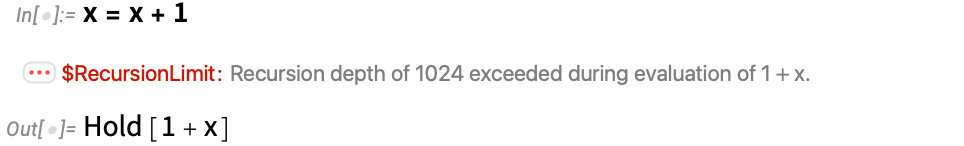
But over the years there’d been increasing evidence that this wasn’t quite adequate, and that for example further processing of the held form (even, for example, formatting it) could in extreme cases end up triggering even infinite cascades of evaluations. So finally—in Version 13.2 at the end of last year—we introduced the beginnings of a new mechanism to cut off “runaway” computations, based on a construct called TerminatedEvaluation:

And from the beginning we wanted to see how to encode within TerminatedEvaluation information about just what evaluation had been terminated. But to do this once again seemed to require having a way to represent the “ongoing process of evaluation”—leading us back to Trace, and making us think about evaluation graphs, causal graphs, etc.
At the beginning x = x + 1 might just have seemed like an irrelevant corner case—and for practical purposes it basically is. But already four decades ago it led me to start thinking not just about the results of computations, but also how their internal processes can be systematically organized. For years, I didn’t really connect this to my work on explicit computational processes like those in systems such as cellular automata. Hints of such connections did start to emerge as I began to try to build computational models of fundamental physics. But looking back I realize that in x = x + 1 there was already in a sense a shadow of what was to come in our Physics Project and in the whole construction of the ruliad.
Because x = x + 1 is something which—like physics and like the ruliad—necessarily generates an ongoing process of computation. One might have thought that the fact that it doesn’t just “give an answer” was in a sense a sign of uselessness. But what we’ve now realized is that our whole existence and experience is based precisely on “living inside a computational process” (which, fortunately for us, hasn’t just “ended with an answer”). Expression evaluation is in its origins intended as a “human-accessible” form of computation. But what we’re now seeing is that its essence also inevitably encompasses computations that are at the core of fundamental physics. And by seeing the correspondence between what might at first appear to be utterly unrelated intellectual directions, we can expect to inform both of them. Which is what I have started to try to do here.
Notes & Thanks
What I’ve described here builds quite directly on some of my recent work, particularly as covered in my books Combinators: A Centennial View and Metamathematics: Physicalization & Foundations. But as I mentioned above, I started thinking about related issues at the beginning of the 1980s in connection with the design of SMP, and I’d like to thank members of the SMP development team for discussions at that time, particularly Chris Cole, Jeff Greif and Tim Shaw. Thanks also to Bruce Smith for his 1990 work on Trace in Wolfram Language, and for encouraging me to think about symbolic representations of computational processes. In much more recent times, I’d particularly like to thank Jonathan Gorard for his extensive conceptual and practical work on multiway systems and their formalism, both in our Physics Project and beyond. Some of the directions described here have (at least indirectly) been discussed in a number of recent Wolfram Language design review livestreams, with particular participation by Ian Ford, Nik Murzin, and Christopher Wolfram, as well as Dan Lichtblau and Itai Seggev. Thanks also to Wolfram Institute fellows Richard Assar and especially Nik Murzin for their help with this piece.