The Drumbeat of Releases Continues…

Just under six months ago (176 days ago, to be precise) we released Version 14.1. Today I’m pleased to announce that we’re releasing Version 14.2, delivering the latest from our R&D pipeline.

This is an exciting time for our technology, both in terms of what we’re now able to implement, and in terms of how our technology is now being used in the world at large. A notable feature of these times is the increasing use of Wolfram Language not only by humans, but also by AIs. And it’s very nice to see that all the effort we’ve put into consistent language design, implementation and documentation over the years is now paying dividends in making Wolfram Language uniquely valuable as a tool for AIs—complementing their own intrinsic capabilities.

But there’s another angle to AI as well. With our Wolfram Notebook Assistant launched last month we’re using AI technology (plus a lot more) to provide what amounts to a conversational interface to Wolfram Language. As I described when we released Wolfram Notebook Assistant, it’s something extremely useful for experts and beginners alike, but ultimately I think its most important consequence will be to accelerate the ability to go from any field X to “computational X”—making use of the whole tower of technology we’ve built around Wolfram Language.

So, what’s new in 14.2? Under the hood there are changes to make Wolfram Notebook Assistant more efficient and more streamlined. But there are also lots of visible extensions and enhancements to the user-visible parts of the Wolfram Language. In total there are 80 completely new functions—along with 177 functions that have been substantially updated.

There are continuations of long-running R&D stories, like additional functionality for video, and additional capabilities around symbolic arrays. Then there are completely new areas of built-in functionality, like game theory. But the largest new development in Version 14.2 is around handling tabular data, and particularly, big tabular data. It’s a whole new subsystem for Wolfram Language, with powerful consequences throughout the system. We’ve been working on it for quite a few years, and we’re excited to be able to release it for the first time in Version 14.2.

Talking of working on new functionality: starting more than seven years ago we pioneered the concept of open software design, livestreaming our software design meetings. And, for example, since the release of Version 14.1, we’ve done 43 software design livestreams, for a total of 46 hours (I’ve also done 73 hours of other livestreams in that time). Some of the functionality that’s now in Version 14.2 we started work on quite a few years ago. But we’ve been livestreaming long enough that pretty much anything that’s now in Version 14.2 we designed live and in public on a livestream at some time or another. It’s hard work doing software design (as you can tell if you watch the livestreams). But it’s always exciting to see the fruits of those efforts come to fruition in the system we’ve been progressively building for so long. And so, today, it’s a pleasure to be able to release Version 14.2 and to let everyone use the things we’ve been working so hard to build.

Notebook Assistant Chat inside Any Notebook

Last month we released the Wolfram Notebook Assistant to “turn words into computation”—and help experts and novices alike make broader and deeper use of Wolfram Language technology. In Version 14.1 the primary way to use Notebook Assistant is through the separate “side chat” Notebook Assistant window. But in Version 14.2 “chat cells” have become a standard feature of any notebook available to anyone with a Notebook Assistant subscription.

Just type ‘ as the first character of any cell, and it’ll become a chat cell:

Now you can start chatting with the Notebook Assistant:

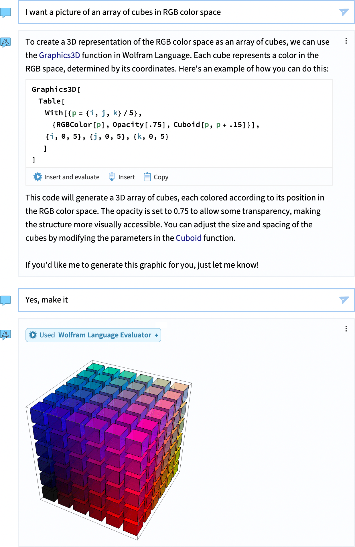
With the side chat you have a “separate channel” for communicating with the Notebook Assistant—that won’t, for example, be saved with your notebook. With chat cells, your chat becomes an integral part of the notebook.

We actually first introduced Chat Notebooks in the middle of 2023—just a few months after the arrival of ChatGPT. Chat Notebooks defined the interface, but at the time, the actual content of chat cells was purely from external LLMs. Now in Version 14.2, chat cells are not limited to separate Chat Notebooks, but are available in any notebook. And by default they make use of the full Notebook Assistant technology stack, which goes far beyond a raw LLM. In addition, once you have a Notebook Assistant + LLM Kit subscription, you can seamlessly use chat cells; no account with external LLM providers is needed.

The chat cell functionality in Version 14.2 inherits all the features of Chat Notebooks. For example, typing ~ in a new cell creates a chat break, that lets you start a “new conversation”. And when you use a chat cell, it’s able to see anything in your notebook up to the most recent chat break. (By the way, when you use Notebook Assistant through side chat it can also see what selection you’ve made in your “focus” notebook.)

By default, chat cells are “talking” to the Notebook Assistant. But if you want, you can also use them to talk to external LLMs, just like in our original Chat Notebook—and there’s a convenient menu to set that up. Of course, if you’re using an external LLM, you don’t have all the technology that’s now in the Notebook Assistant, and unless you’re doing LLM research, you’ll typically find it much more useful and valuable to use chat cells in their default configuration—talking to the Notebook Assistant.

Bring Us Your Gigabytes! Introducing Tabular

Lists, associations, datasets. These are very flexible ways to represent structured collections of data in the Wolfram Language. But now in Version 14.2 there’s another: Tabular. Tabular provides a very streamlined and efficient way to handle tables of data laid out in rows and columns. And when we say “efficient” we mean that it can routinely juggle gigabytes of data or more, both in core and out of core.

Let’s do an example. Let’s start off by importing some tabular data:

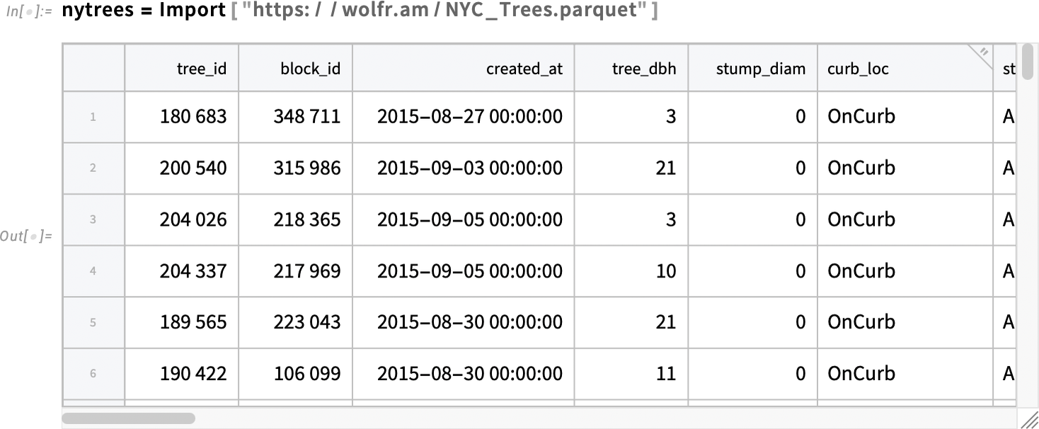
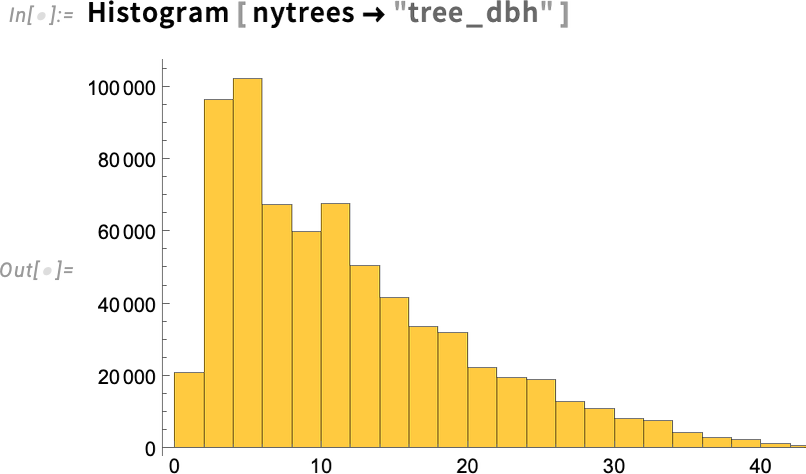
This is data on trees in New York City, 683,788 of them, each with 45 properties (sometimes missing). Tabular introduces a variety of new ideas. One of them is treating tabular columns much like variables. Here we’re using this to make a histogram of the values of the "tree_dbh" column in this Tabular:

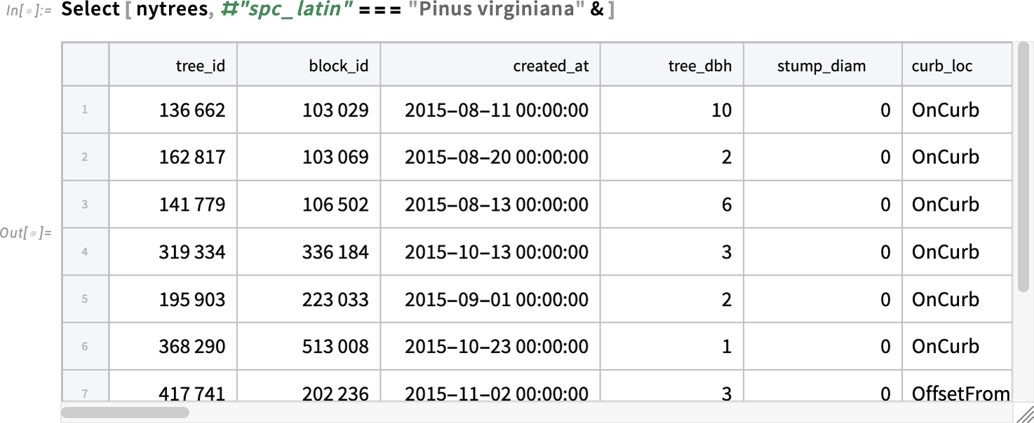
You can think of a Tabular as being like an optimized form of a list of associations, where each row consists of an association whose keys are column names. Functions like Select then just work on Tabular:

Length gives the number of rows:

CountsBy treats the Tabular as a list of associations, extracting the value associated with the key "spc_latin" (“Latin species”) in each association, and counting how many times that value occurs ("spc_latin" here is short for #"spc_latin"&):

To get the names of the columns we can use the new function ColumnKeys:

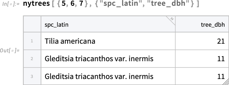
Viewing Tabular as being like a list of associations we can extract parts—giving first a specification of rows, and then a specification of columns:

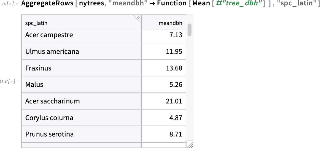
There are lots of new operations that we’ve been able to introduce now that we have Tabular. An example is AggregrateRows, which constructs a new Tabular from a given Tabular by aggregating groups of rows, in this case ones with the same value of "spc_latin", and then applying a function to those rows, in this case finding the mean value of "tree_dbh":

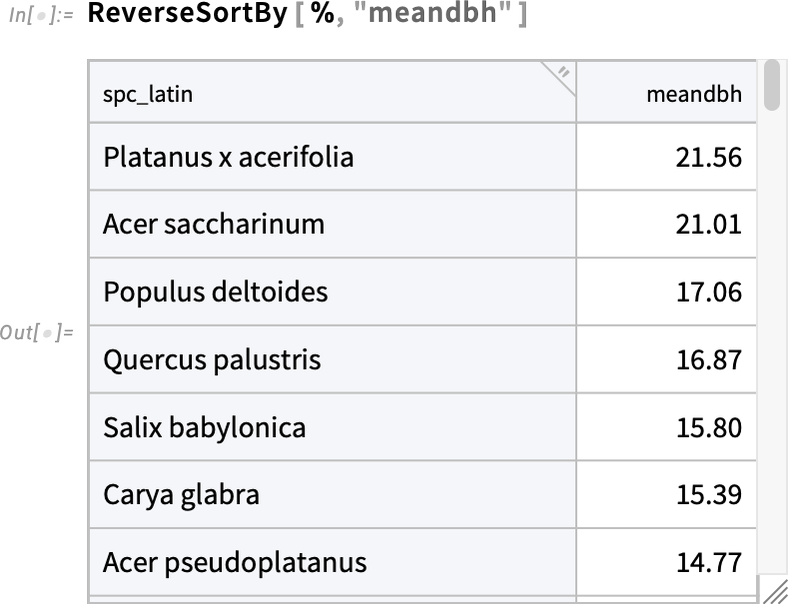
An operation like ReverseSortBy then “just works” on this table, here reverse sorting by the value of "meandbh":

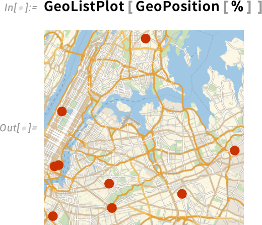
Here we’re making an ordinary matrix out of a small slice of data from our Tabular:

And now we can plot the result, giving the positions of Virginia pine trees in New York City:

When should you use a Tabular, rather than, say a Dataset? Tabular is specifically set up for data that is arranged in rows and columns—and it supports many powerful operations that make sense for data in this “rectangular” form. Dataset is more general; it can have an arbitrary hierarchy of data dimensions, and so can’t in general support all the “rectangular” data operations of Tabular. In addition, by being specialized for “rectangular” data, Tabular can also be much more efficient, and indeed we’re making use of the latest type-specific methods for large-scale data handling.

If you use TabularStructure you can see some of what lets Tabular be so efficient. Every column is treated as data of a specific type (and, yes, the types are consistent with the ones in the Wolfram Language compiler). And there’s streamlined treatment of missing data (with several new functions added specifically to handle this):

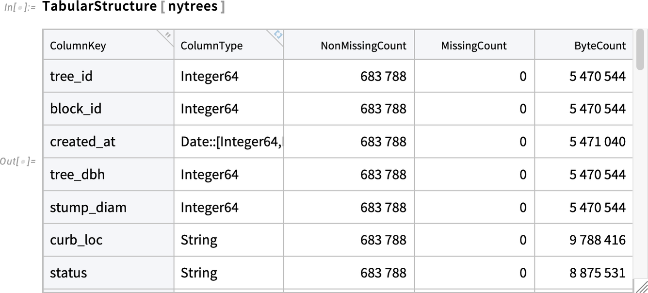
What we’ve seen so far is Tabular operating with “in-core” data. But you can quite transparently also use Tabular on out-of-core data, for example data stored in a relational database.

Here’s an example of what this looks like:

It’s a tabular that points to a table in a relational database. It doesn’t by default explicitly display the data in the Tabular (and in fact it doesn’t even get it into memory—because it might be huge and might be changing quickly as well). But you can still specify operations just like on any other Tabular. This finds out what columns are there:

And this specifies an operation, giving the result as a symbolic out-of-core Tabular object:

You can “resolve” this, and get an explicit in-memory Tabular using ToMemory:

Manipulating Data in Tabular

Let’s say you’ve got a Tabular—like this one based on penguins:

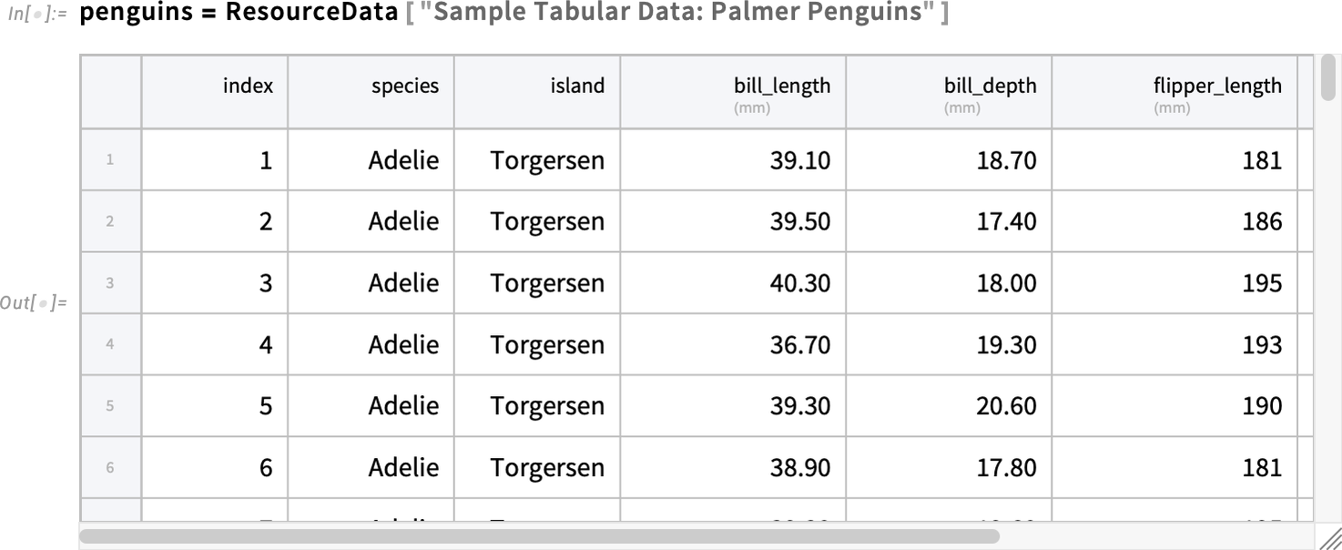
There are lots of operations you can do that manipulate the data in this Tabular in a structured way—giving you back another Tabular. For example, you could just take the last 2 rows of the Tabular:

Or you could sample 3 random rows:

Other operations depend on the actual content of the Tabular. And because you can treat each row like an association, you can set up functions that effectively refer to elements by their column names:

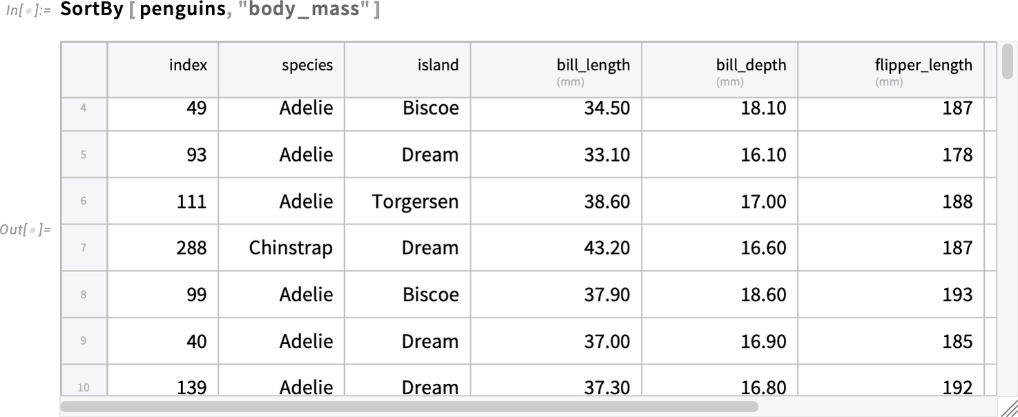
Note that we can always use #[name] to refer to elements in a column. If name is an alphanumeric string then we can also use the shorthand #name. And for other strings, we can use #"name". Some functions let you just use "name" to indicate the function #["name"]:

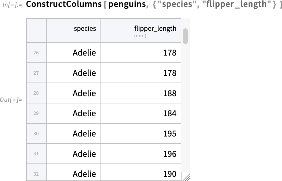
So far we’ve talked only about arranging or selecting rows in a Tabular. What about columns? Here’s how we can construct a tabular that has just two of the columns from our original Tabular:

What if we don’t just want existing columns, but instead want new columns that are functions of these? ConstructColumns lets us define new columns, giving their names and the functions to be used to compute values in them:

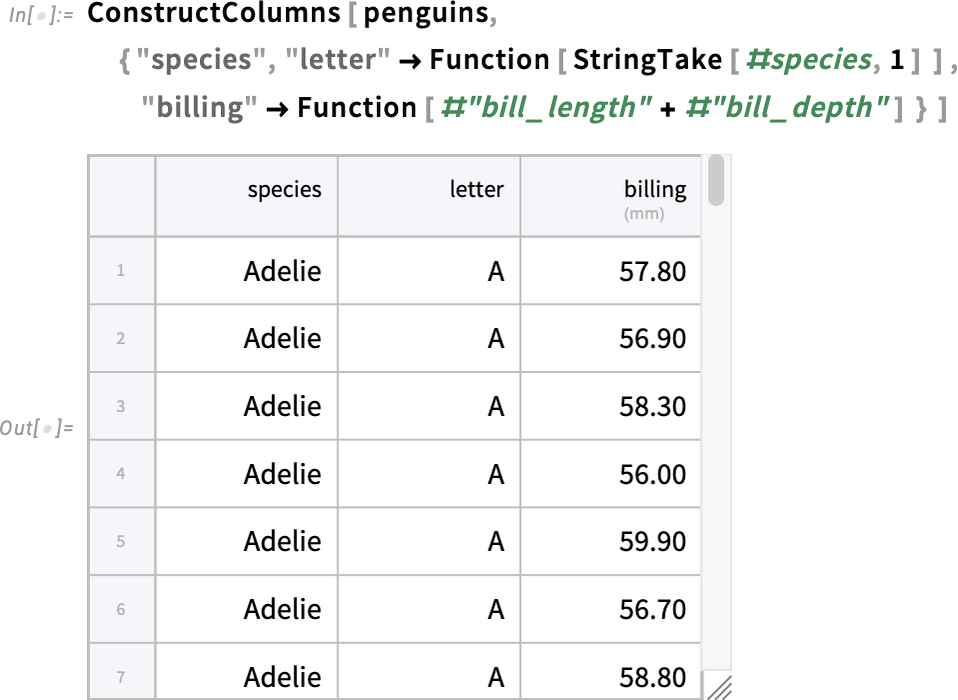
(Note the trick of writing out Function to avoid having to put parentheses, as in "letter"(StringTake["species",1]&).)

ConstructColumns lets you take an existing Tabular and construct a new one. TransformColumns lets you transform columns in an existing Tabular, here replacing species names by their first letters:

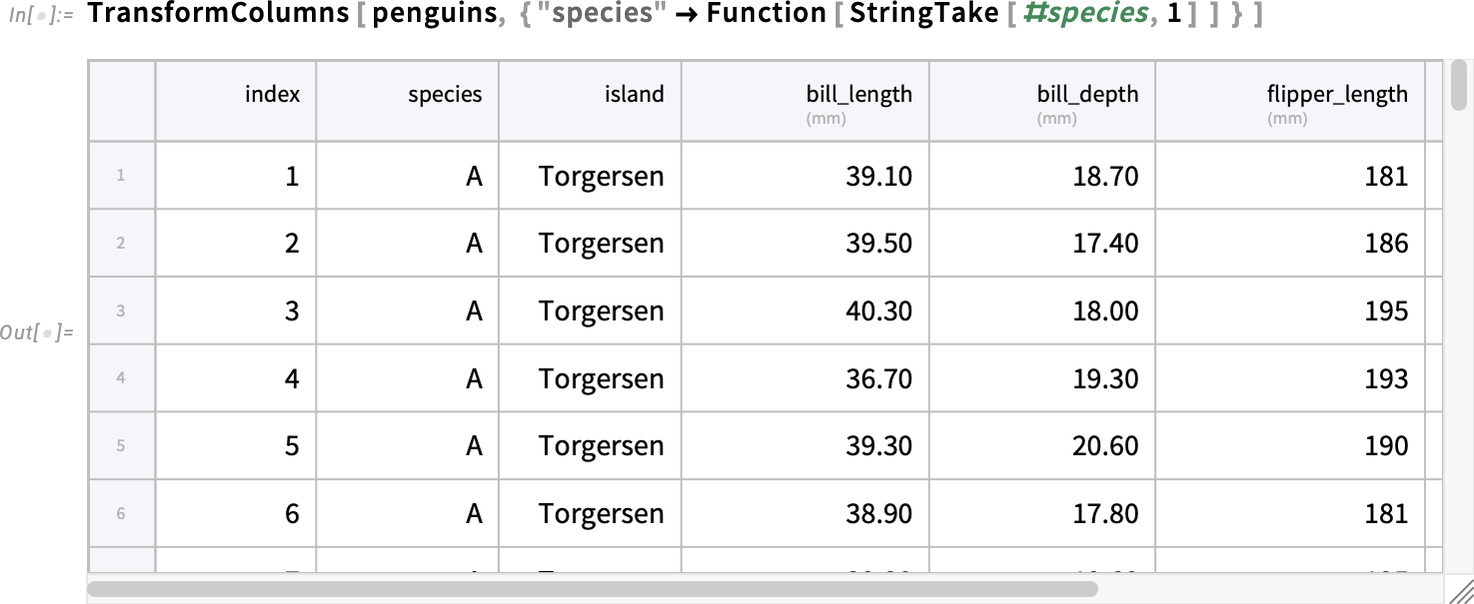
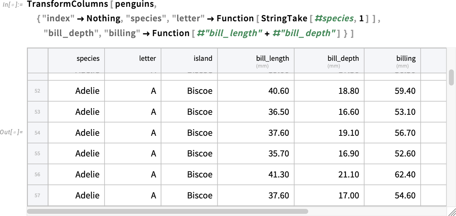
TransformColumns also lets you add new columns, specifying the content of the columns just like in ConstructColumns. But where does TransformColumns put your new columns? By default, they go at the end, after all existing columns. But if you specifically list an existing column, that’ll be used as a marker to determine where to put the new column ("name"Nothing removes a column):

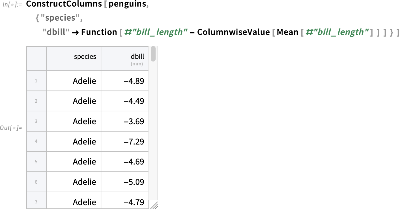
Everything we’ve seen so far operates separately on each row of a Tabular. But what if we want to “gulp in” a whole column to use in our computation—say, for example, computing the mean of a whole column, then subtracting it from each value. ColumnwiseValue lets you do this, by supplying to the function (here Mean) a list of all the values in whatever column or columns you specify:

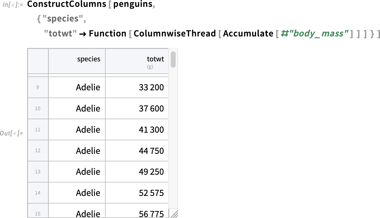
ColumnwiseValue effectively lets you compute a scalar value by applying a function to a whole column. There’s also ColumnwiseThread, which lets you compute a list of values, that will in effect be “threaded” into a column. Here we’re creating a column from a list of accumulated values:

By the way, as we’ll discuss below, if you’ve externally generated a list of values (of the right length) that you want to use as a column, you can do that directly by using InsertColumns.

There’s another concept that’s very useful in practice in working with tabular data, and that’s grouping. In our penguin data, we’ve got an individual row for each penguin of each species. But what if we want instead to aggregate all the penguins of a given species, for example computing their average body mass? Well, we can do this with AggregateRows. AggregateRows works like ConstructColumns in the sense that you specify columns and their contents. But unlike ConstructColumns it creates new “aggregated” rows:

What is that first column here? The gray background of its entries indicates that it’s what we call a “key column”: a column whose entries (perhaps together with other key columns) can be used to reference rows. And later, we’ll see how you can use RowKey to indicate a row by giving a value from a key column:

But let’s go on with our aggregation efforts. Let’s say that we want to group not just by species, but also by island. Here’s how we can do that with AggregateRows:

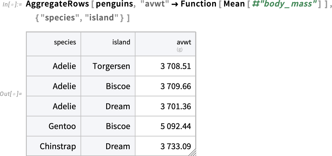
In a sense what we have here is a table whose rows are specified by pairs of values (here “species” and “island”). But it’s often convenient to “pivot” things so that these values are used respectively for rows and for columns. And you can do that with PivotTable:

Note the —’s, which indicate missing values; apparently there are no Gentoo penguins on Dream island, etc.

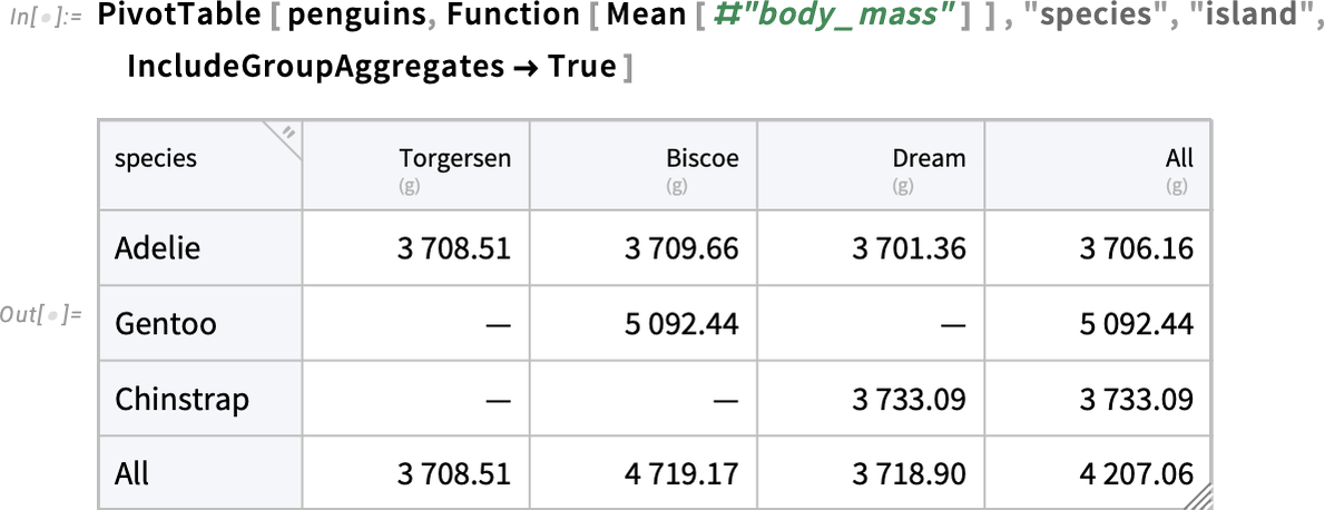
PivotTable normally gives exactly the same data as AggregateRows, but in a rearranged form. One additional feature of PivotTable is the option IncludeGroupAggregates which includes All entries that aggregate across each type of group:

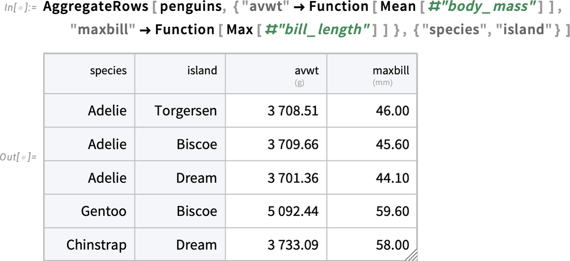
If you have multiple functions that you’re computing, AggregateRows will just give them as separate columns:

PivotTable can also deal with multiple functions—by creating columns with “extended keys”:

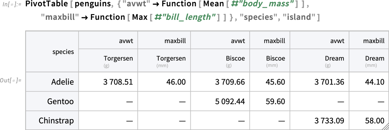
And now you can use RowKey and ExtendedKey to refer to elements of the resulting Tabular:

Getting Data into Tabular

We’ve seen some of the things you can do when you have data as a Tabular. But how does one get data into a Tabular? There are several ways. The first is just to convert from structures like lists and associations. The second is to import from a file, say a CSV or XLSX (or, for larger amounts of data, Parquet)—or from an external data store (S3, Dropbox, etc.). And the third is to connect to a database. You can also get data for Tabular directly from the Wolfram Knowledgebase or from the Wolfram Data Repository.

Here’s how you can convert a list of lists into a Tabular:

And here’s how you can convert back:

It works with sparse arrays too, here instantly creating a million-row Tabular

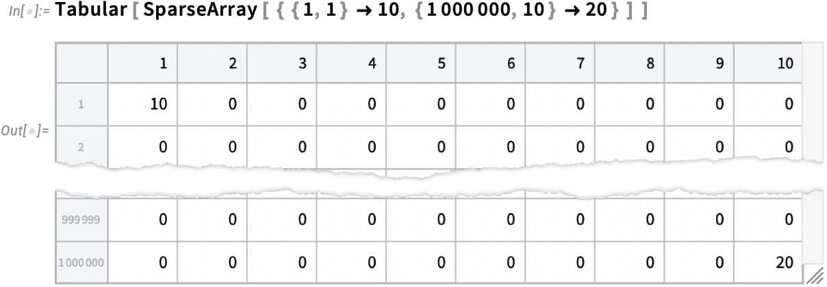
that takes 80 MB to store:

Here’s what happens with a list of associations:

You can get the same Tabular by entering its data and its column names separately:

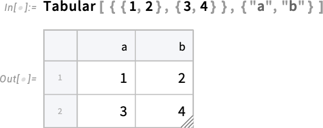
By the way, you can convert a Tabular to a Dataset

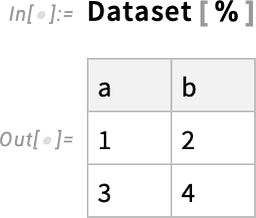
and in this simple case you can convert it back to a Tabular too:

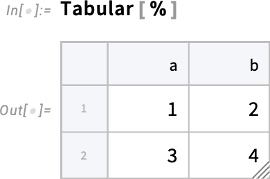
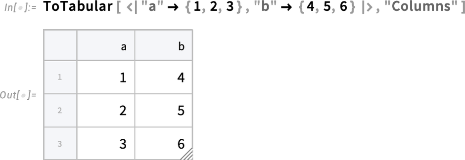
In general, though, there are all sorts of options for how to convert lists, datasets, etc. to Tabular objects—and ToTabular is set up to let you control these. For example, you can use ToTabular to create a Tabular from columns rather than rows:

How about external data? In Version 14.2 Import now supports a "Tabular" element for tabular data formats. So, for example, given a CSV file

Import can immediately import it as a Tabular:

This works very efficiently even for huge CSV files with millions of entries. It also does well at automatically identifying column names and headers. The same kind of thing works with more structured files, like ones from spreadsheets and statistical data formats. And it also works with modern columnar storage formats like Parquet, ORC and Arrow.

Import transparently handles both ordinary files, and URLs (and URIs), requesting authentication if needed. In Version 14.2 we’re adding the new concept of DataConnectionObject, which provides a symbolic representation of remote data, essentially encapsulating all the details of how to get the data. So, for example, here’s a DataConnectionObject for an S3 bucket, whose contents we can immediately import:

(In Version 14.2 we’re supporting Amazon S3, Azure Blob Storage, Dropbox, IPFS—with many more to come. And we’re also planning support for data warehouse connections, APIs, etc.)

But what about data that’s too big—or too fast-changing—to make sense to explicitly import? An important feature of Tabular (mentioned above) is that it can transparently handle external data, for example in relational databases.

Here’s a reference to a large external database:

This defines a Tabular that points to a table in the external database:

We can ask for the dimensions of the Tabular—and we see that it has 158 million rows:

The table we’re looking at happens to be all the line-oriented data in OpenStreetMap. Here are the first 3 rows and 10 columns:

Most operations on the Tabular will now actually get done in the external database. Here we’re asking to select rows whose “name” field contains "Wolfram":

The actual computation is only done when we use ToMemory, and in this case (because there’s a lot of data in the database) it takes a little while. But soon we get the result, as a Tabular:

And we learn that there are 58 Wolfram-named items in the database:

Another source of data for Tabular is the built-in Wolfram Knowledgebase. In Version 14.2 EntityValue supports direct output in Tabular form:

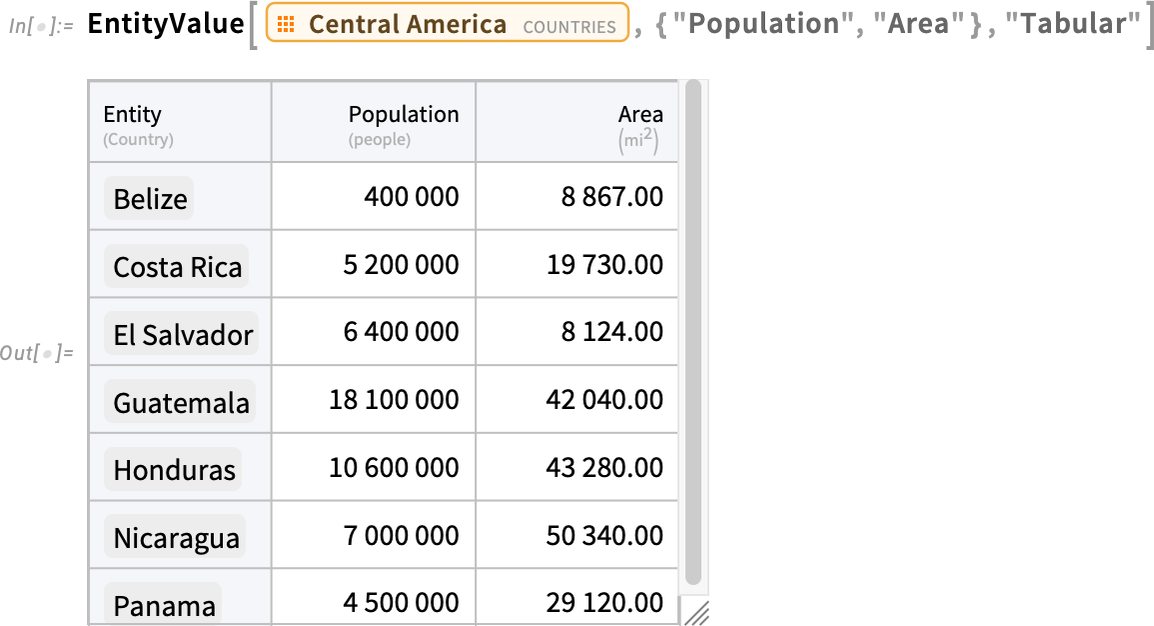
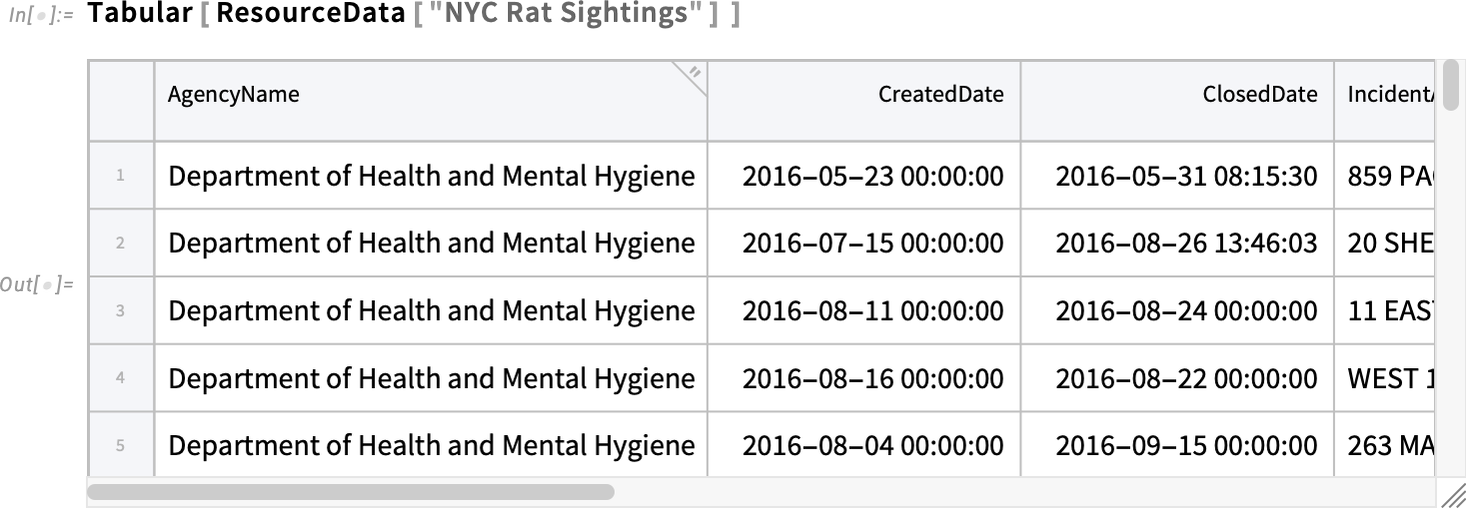
The Wolfram Knowledgebase provides lots of good examples of data for Tabular. And the same is true of the Wolfram Data Repository—where you can typically just apply Tabular to get data in Tabular form:

Cleaning Data for Tabular

In many ways it’s the bane of data science. Yes, data is in digital form. But it’s not clean; it’s not computable. The Wolfram Language has long been a uniquely powerful tool for flexibly cleaning data (and, for example, for advancing through the ten levels of making data computable that I defined some years ago).

But now, in Version 14.2, with Tabular, we have a whole new collection of streamlined capabilities for cleaning data. Let’s start by importing some data “from the wild” (and, actually, this example is cleaner than many):

(By the way, if there was really crazy stuff in the file, we might have wanted to use the option MissingValuePattern to specify a pattern that would just immediately replace the crazy stuff with Missing[…].)

OK, but let’s start by surveying what came in here from our file, using TabularStructure:

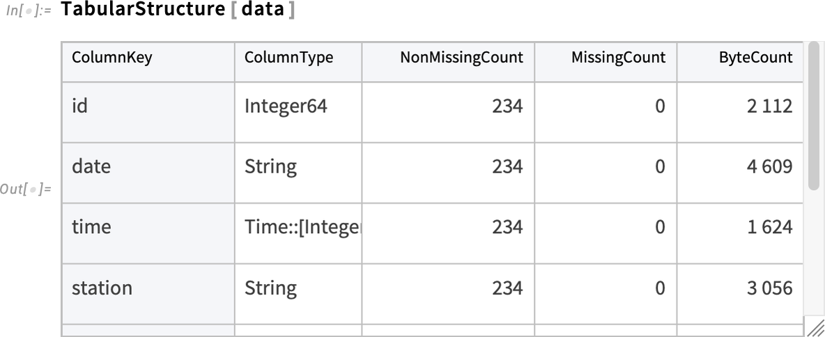
We see that Import successfully managed to identify the basic type of data in most of the columns—though for example it can’t tell if numbers are just numbers or are representing quantities with units, etc. And it also identifies that some number of entries in some columns are “missing”.

As a first step in data cleaning, let’s get rid of what seems like an irrelevant "id" column:

Next, we see that the elements in the first column are being identified as strings—but they’re really dates, and they should be combined with the times in the second column. We can do this with TransformColumns, removing what’s now an “extra column” by replacing it with Nothing:

Looking at the various numerical columns, we see that they’re really quantities that should have units. But first, for convenience, let’s rename the last two columns:

Now let’s turn the numerical columns into columns of quantities with units, and, while we’re at it, also convert from °C to °F:

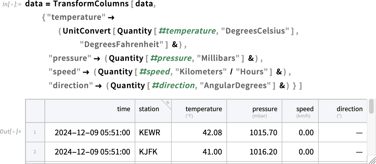
Here’s how we can now plot the temperature as a function of time:

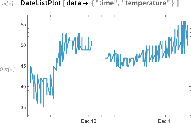
There’s a lot of wiggling there. And looking at the data we see that we’re getting temperature values from several different weather stations. This selects data from a single station:

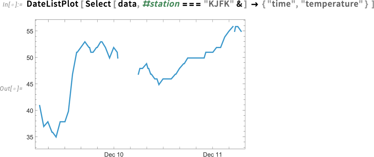
What’s the break in the curve? If we just scroll to that part of the tabular we’ll see that it’s because of missing data:

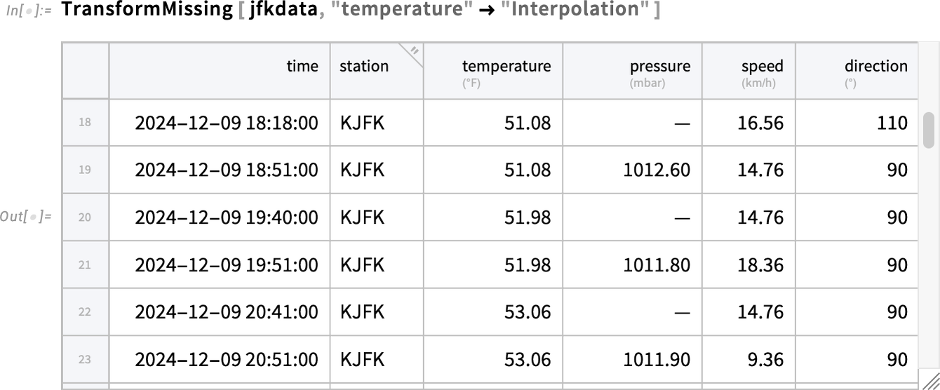
So what can we do about this? Well, there’s a powerful function TransformMissing that provides many options. Here we’re asking it to interpolate to fill in missing temperature values:

And now there are no gaps, but, slightly mysteriously, the whole plot extends further:

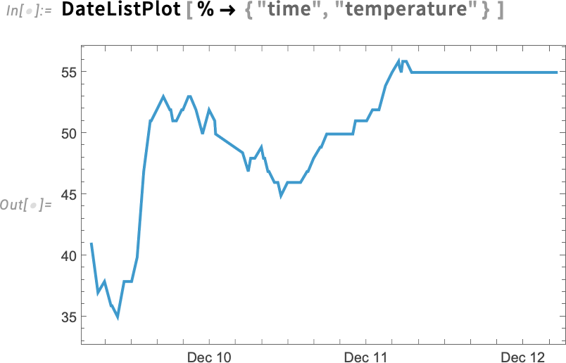
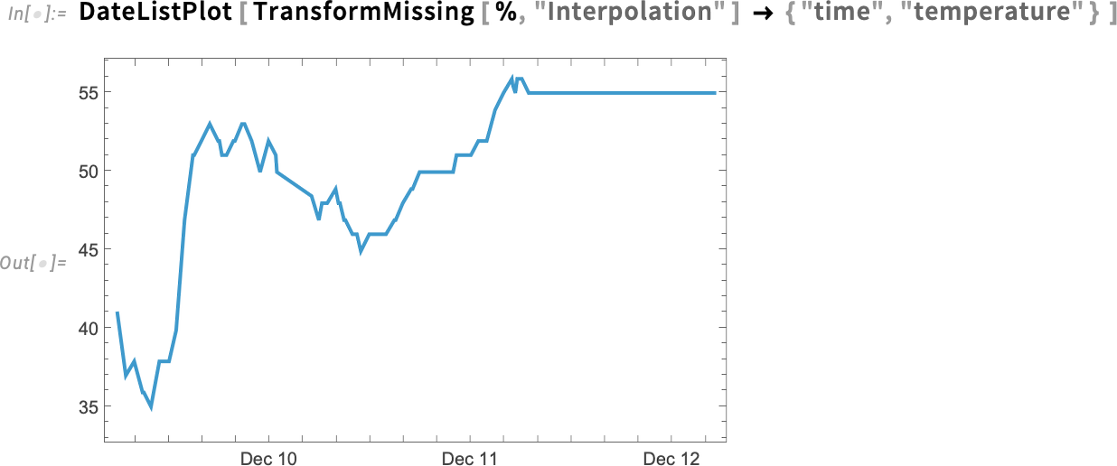
The reason is that it’s interpolating even in cases where basically nothing was measured. We can remove those rows using Discard:

And now we won’t have that “overhang” at the end:

Sometimes there’ll explicitly be data that’s missing; sometimes (more insidiously) the data will just be wrong. Let’s look at the histogram of pressure values for our data:

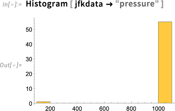
Oops. What are those small values? Presumably they’re wrong. (Perhaps they were transcription errors?) We can remove such “anomalous” values by using TransformAnomalies. Here we’re telling it to just completely trim out any row where the pressure was “anomalous”:

We can also get TransformAnomalies to try to “fix” the data. Here we’re just replacing any anomalous pressure by the previous pressure listed in the tabular:

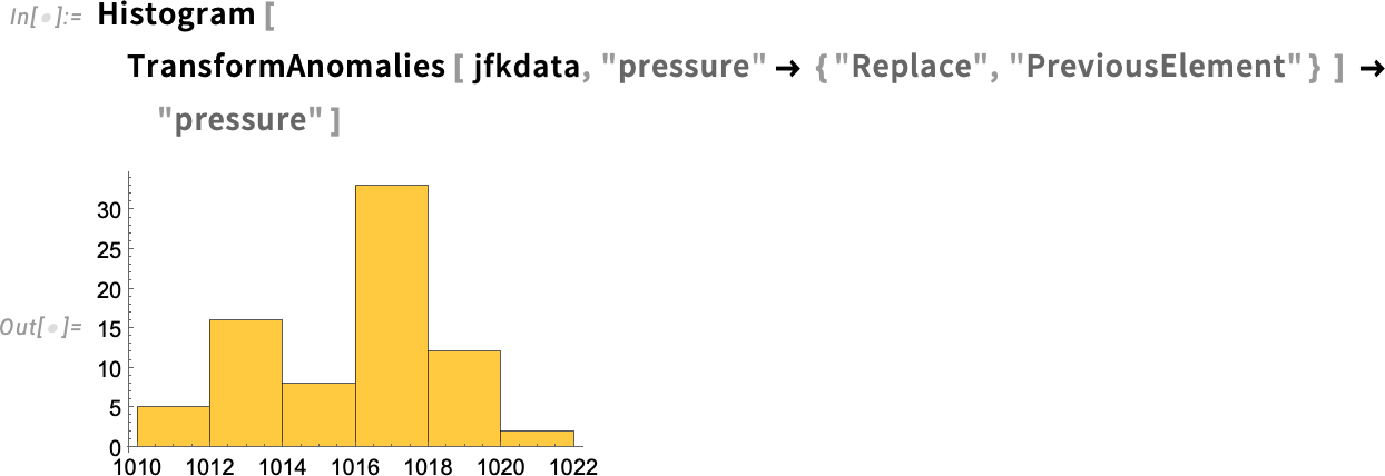
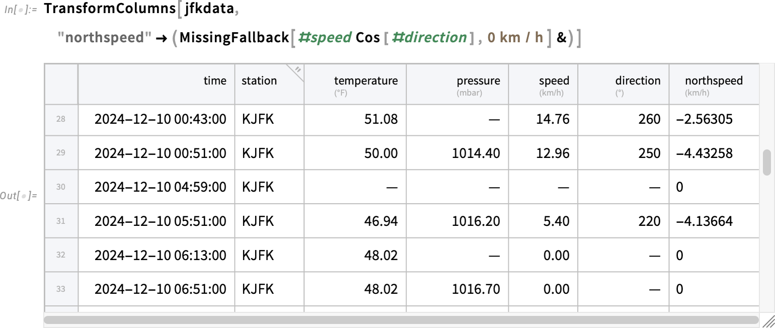
You can also tell TransformAnomalies to “flag” any anomalous value and make it “missing”. But, if we’ve got missing values what then happens if we try to do computations on them? That’s where MissingFallback comes in. It’s fundamentally a very simple function—that just returns its first non-missing argument:

But even though it’s simple, it’s important in making it easy to handle missing values. So, for example, this computes a “northspeed”, falling back to 0 if data needed for the computation is missing:

The Structure of Tabular

We’ve said that a Tabular is “like” a list of associations. And, indeed, if you apply Normal to it, that’s what you’ll get:

But internally Tabular is stored in a much more compact and efficient way. And it’s useful to know something about this, so you can manipulate Tabular objects without having to “take them apart” into things like lists and associations. Here’s our basic sample Tabular:

What happens if we extract a row? Well, we get a TabularRow object:

If we apply Normal, we get an association:

Here’s what happens if we instead extract a column:

Now Normal gives a list:

We can create a TabularColumn from a list:

Now we can use InsertColumns to insert a symbolic column like this into an existing Tabular (including the "b" tells InsertColumns to insert the new column after the “b” column):

But what actually is a Tabular inside? Let’s look at the example:

TabularStructure gives us a summary of the internal structure here:

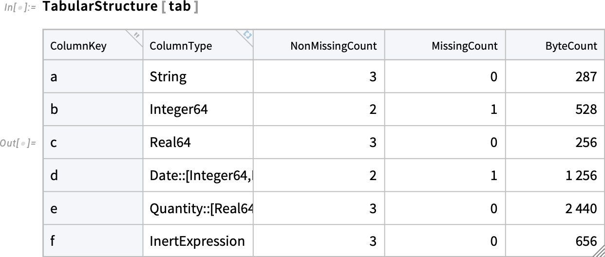
The first thing to notice is that everything is stated in terms of columns, reflecting the fact that Tabular is a fundamentally column-oriented construct. And part of what makes Tabular so efficient is then that within a column everything is uniform, in the sense that all the values are the same type of data. In addition, for things like quantities and dates, we factor the data so that what’s actually stored internally in the column is just a list of numbers, with a single copy of “metadata information” on how to interpret them.

And, yes, all this has a big effect. Like here’s the size in bytes of our New York trees Tabular from above:

But if we turn it into a list of associations using Normal, the result is about 14x larger:

OK, but what are those “column types” in the tabular structure? ColumnTypes gives a list of them:

These are low-level types of the kind used in the Wolfram Language compiler. And part of what knowing these does is that it immediately tells us what operations we can do on a particular column. And that’s useful both in low-level processing, and in things like knowing what kind of visualization might be possible.

When Import imports data from something like a CSV file, it tries to infer what type each column is. But sometimes (as we mentioned above) you’ll want to “cast” a column to a different type, specifying the “destination type” using Wolfram Language type description. So, for example, this casts column “b” to a 32-bit real number, and column “c” to units of meters:

By the way, when a Tabular is displayed in a notebook, the column headers indicate the types of data in the corresponding columns. So in this case, there’s a little in the first column to indicate that it contains strings. Numbers and dates basically just “show what they are”. Quantities have their units indicated. And general symbolic expressions (like column “f” here) are indicated with . (If you hover over a column header, it gives you more detail about the types.)

The next thing to discuss is missing data. Tabular always treats columns as being of a uniform type, but keeps an overall map of where values are missing. If you extract the column you’ll see a symbolic Missing:

But if you operate on the tabular column directly it’ll just behave as if the missing data is, well, missing:

By the way, if you’re bringing in data “from the wild”, Import will attempt to automatically infer the right type for each column. It knows how to deal with common anomalies in the input data, like NaN or null in a column of numbers. But if there are other weird things—like, say, notfound in the middle of a column of numbers—you can tell Import to turn such things into ordinary missing data by giving them as settings for the option MissingValuePattern.

There are a couple more subtleties to discuss in connection with the structure of Tabular objects. The first is the notion of extended keys. Let’s say we have the following Tabular:

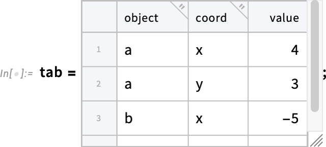
We can “pivot this to columns” so that the values x and y become column headers, but “under” the overall column header “value”:

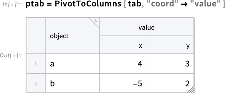
But what is the structure of this Tabular? We can use ColumnKeys to find out:

You can now use these extended keys as indices for the Tabular:

In this particular case, because the “subkeys” "x" and "y" are unique, we can just use those, without including the other part of the extended key:

Our final subtlety (for now) is somewhat related. It concerns key columns. Normally the way we specify a row in a Tabular object is just by giving its position. But if the values of a particular column happen to be unique, then we can use those instead to specify a row. Consider this Tabular:

The fruit column has the feature that each entry appears only once—so we can create a Tabular that uses this column as a key column:

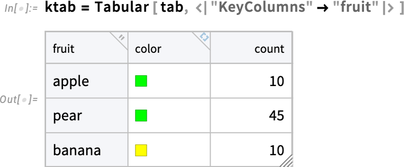
Notice that the numbers for rows have now disappeared, and the key column is indicated with a gray background. In this Tabular, you can then reference a particular row using for example RowKey:

Equivalently, you can also use an association with the column name:

What if the values in a single column are not sufficient to uniquely specify a row, but several columns together are? (In a real-world example, say one column has first names, and another has last names, and another has dates of birth.) Well, then you can designate all those columns as key columns:

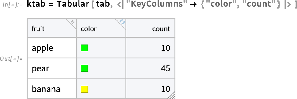
And once you’ve done that, you can reference a row by giving the values in all the key columns:

Tabular Everywhere

Tabular provides an important new way to represent structured data in the Wolfram Language. It’s powerful in its own right, but what makes it even more powerful is how it integrates with all the other capabilities in the Wolfram Language. Many functions just immediately work with Tabular. But in Version 14.2 hundreds have been enhanced to make use of the special features of Tabular.

Most often, it’s to be able to operate directly on columns in a Tabular. So, for example, given the Tabular

we can immediately make a visualization based on two of the columns:

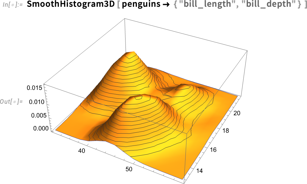
If one of the columns has categorical data, we’ll recognize that, and plot it accordingly:

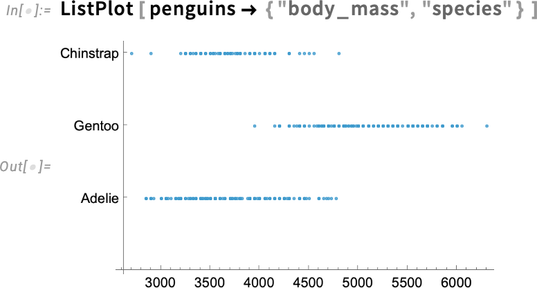
Another area where Tabular can immediately be used is machine learning. So, for example, this creates a classifier function that will attempt to determine the species of a penguin from other data about it:

Now we can use this classifier function to predict species from other data about a penguin:

We can also take the whole Tabular and make a feature space plot, labeling with species:

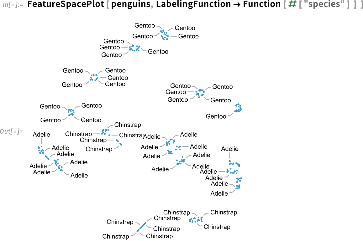
Or we could “learn the distribution of possible penguins”

and randomly generate 3 “fictitious penguins” from this distribution:

Algebra with Symbolic Arrays

One of the major innovations of Version 14.1 was the introduction of symbolic arrays—and the ability to create expressions involving vector, matrix and array variables, and to take derivatives of them. In Version 14.2 we’re taking the idea of computing with symbolic arrays a step further—for the first time systematically automating what has in the past been the manual process of doing algebra with symbolic arrays, and simplifying expressions involving symbolic arrays.

Let’s start by talking about ArrayExpand. Our longstanding function Expand just deals with expanding ordinary multiplication, effectively of scalars—so in this case it does nothing:

But in Version 14.2 we also have ArrayExpand which will do the expansion:

ArrayExpand deals with many generalizations of multiplication that aren’t commutative:

In an example like this, we really don’t need to know anything about a and b. But sometimes we can’t do the expansion without, for example, knowing their dimensions. One way to specify those dimensions is as a condition in ArrayExpand:

An alternative is to use an explicit symbolic array variable:

In addition to expanding generalized products using ArrayExpand, Version 14.2 also supports general simplification of symbolic array expressions:

The function ArraySimplify will specifically do simplification on symbolic arrays, while leaving other parts of expressions unchanged. Version 14.2 supports many kinds of array simplifications:

We could do these simplifications without knowing anything about the dimensions of a and b. But sometimes we can’t go as far without knowing these. For example, if we don’t know the dimensions we get:

But with the dimensions we can explicitly simplify this to an n×n identity matrix:

ArraySimplify can also take account of the symmetries of arrays. For example, let’s set up a symbolic symmetric matrix:

And now ArraySimplify can immediately resolve this:

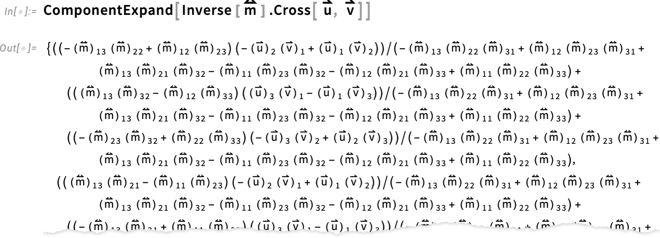
The ability to do algebraic operations on complete arrays in symbolic form is very powerful. But sometimes it’s also important to look at individual components of arrays. And in Version 14.2 we’ve added ComponentExpand to let you get components of arrays in symbolic form.

So, for example this takes a 2-component vector and writes it out as an explicit list with two symbolic components:

Underneath, those components are represented using Indexed:

Here’s the determinant of a 3×3 matrix, written out in terms of symbolic components:

And here’s a matrix power:

Given 3D vectors and we can also for example form the cross product

and we can then go ahead and dot it into an inverse matrix:

Language Tune-Ups

As a daily user of the Wolfram Language I’m very pleased with how smoothly I find I can translate computational ideas into code. But the more we’ve made it easy to do, the more we can see new places where we can polish the language further. And in Version 14.2—like every version before it—we’ve added a number of “language tune-ups”.

A simple one—whose utility becomes particularly clear with Tabular—is Discard. You can think of it as a complement to Select: it discards elements according to the criterion you specify:

And along with adding Discard, we’ve also enhanced Select. Normally, Select just gives a list of the elements it selects. But in Version 14.2 you can specify other results. Here we’re asking for the “index” (i.e. position) of the elements that NumberQ is selecting:

Something that can be helpful in dealing with very large amounts of data is getting a bit vector data structure from Select (and Discard), that provides a bit mask of which elements are selected or not:

By the way, here’s how you can ask for multiple results from Select and Discard:

In talking about Tabular we already mentioned MissingFallback. Another function related to code robustification and error handling is the new function Failsafe. Let’s say you’ve got a list which contains some “failed” elements. If you map a function f over that list, it’ll apply itself to the failure elements just as to everything else:

But quite possibly f wasn’t set up to deal with these kinds of failure inputs. And that’s where Failsafe comes in. Because Failsafe[f][x] is defined to give f[x] if x is not a failure, and to just return the failure if it is. So now we can map f across our list with impunity, knowing it’ll never be fed failure input:

Talking of tricky error cases, another new function in Version 14.2 is HoldCompleteForm. HoldForm lets you display an expression without doing ordinary evaluation of the expression. But—like Hold—it still allows certain transformations to get made. HoldCompleteForm—like HoldComplete—prevents all these transformations. So while HoldForm gets a bit confused here when the sequence “resolves”

HoldCompleteForm just completely holds and displays the sequence:

Another piece of polish added in Version 14.2 concerns Counts. I often find myself wanting to count elements in a list, including getting 0 when a certain element is missing. By default, Counts just counts elements that are present:

But in Version 14.2 we’ve added a second argument that lets you give a complete list of all the elements you want to count—even if they happen to be absent from the list:

As a final example of language tune-up in Version 14.2 I’ll mention AssociationComap. In Version 14.0 we introduced Comap as a “co-” (as in “co-functor”, etc.) analog of Map:

In Version 14.2 we’re introducing AssociationComap—the “co-” version of AssociationMap:

Think of it as a nice way to make labeled tables of things, as in:

Brightening Our Colors; Spiffing Up for 2025

In 2014—for Version 10.0—we did a major overhaul of the default colors for all our graphics and visualization functions, coming up with what we felt was a good solution. (And as we’ve just noticed, somewhat bizarrely, it turned out that in the years that followed, many of the graphics and visualization libraries out there seemed to copy what we did!) Well, a decade has now passed, visual expectations (and display technologies) have changed, and we decided it was time to spiff up our colors for 2025.

Here’s what a typical plot looked like in Versions 10.0 through 14.1:

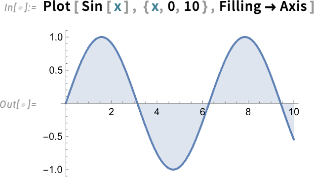
And here’s the same plot in Version 14.2:

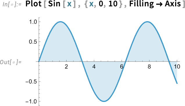
By design, it’s still completely recognizable, but it’s got a little extra zing to it.

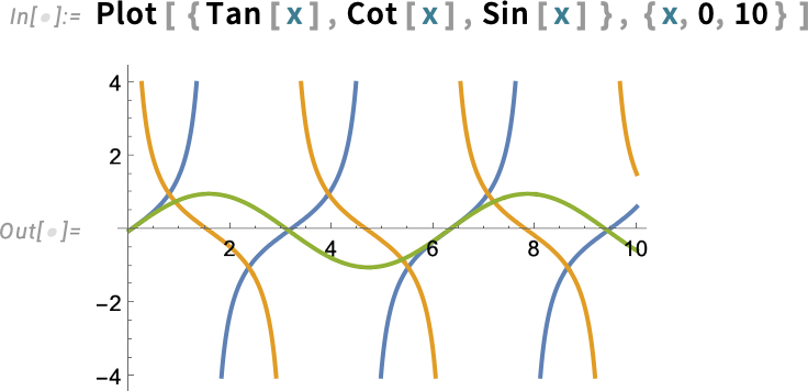
With more curves, there are more colors. Here’s the old version:

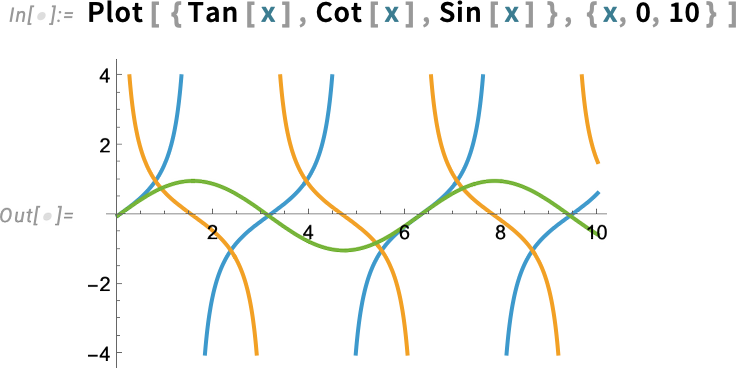
And here’s the new version:

Histograms are brighter too. The old:

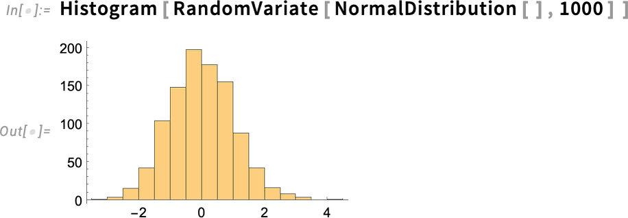
And the new:

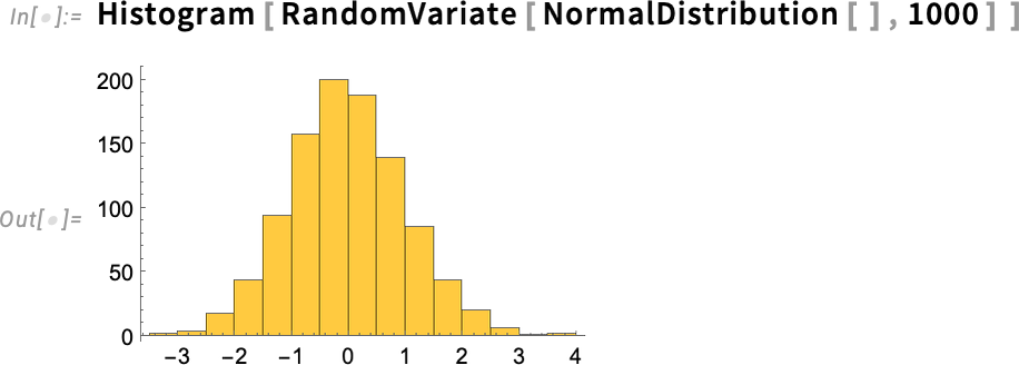
Here’s the comparison between old (“2014”) and new (“2025”) colors:

It’s subtle, but it makes a difference. I have to say that increasingly over the past few years, I’ve felt I had to tweak the colors in almost every Wolfram Language image I’ve published. But I’m excited to say that with the new colors that urge has gone away—and I can just use our default colors again!

LLM Streamlining & Streaming

We first introduced programmatic access to LLMs in Wolfram Language in the middle of 2023, with functions like LLMFunction and LLMSynthesize. At that time, these functions needed access to external LLM services. But with the release last month of LLM Kit (along with Wolfram Notebook Assistant) we’ve made these functions seamlessly available for everyone with a Notebook Assistant + LLM Kit subscription. Once you have your subscription, you can use programmatic LLM functions anywhere and everywhere in Version 14.2 without any further set up.

There are also two new functions: LLMSynthesizeSubmit and ChatSubmit. Both are concerned with letting you get incremental results from LLMs (and, yes, that’s important, at least for now, because LLMs can be quite slow). Like CloudSubmit and URLSubmit, LLMSynthesizeSubmit and ChatSubmit are asynchronous functions: you call them to start something that will call an appropriate handler function whenever a certain specified event occurs.

Both LLMSynthesizeSubmit and ChatSubmit support a whole variety of events. An example is "ContentChunkReceived": an event that occurs when there’s a chunk of content received from the LLM.

Here’s how one can use that:

The LLMSynthesizeSubmit returns a TaskObject, but then starts to synthesize text in response to the prompt you’ve given, calling the handler function you specified every time a chunk of text comes in. After a few moments, the LLM will have finished its process of synthesizing text, and if you ask for the value of c you’ll see each of the chunks it produced:

Let’s try this again, but now setting up a dynamic display for a string s and then running LLMSynthesizeSubmit to accumulate the synthesized text into this string:

ChatSubmit is the analog of ChatEvaluate, but asynchronous—and you can use it to create a full chat experience, in which content is streaming into your notebook as soon as the LLM (or tools called by the LLM) generate it.

Streamlining Parallel Computation: Launch All the Machines!

For nearly 20 years we’ve had a streamlined capability to do parallel computation in Wolfram Language, using functions like ParallelMap, ParallelTable and Parallelize. The parallel computation can happen on multiple cores on a single machine, or across many machines on a network. (And, for example, in my own current setup I have 7 machines right now with a total of 204 cores. )

In the past few years, partly responding to the increasing number of cores typically available on individual machines, we’ve been progressively streamlining the way that parallel computation is provisioned. And in Version 14.2 we’ve, yes, parallelized the provisioning of parallel computation. Which means, for example, that my 7 machines all start their parallel kernels in parallel—so that the whole process is now finished in a matter of seconds, rather than potentially taking minutes, as it did before:

Another new feature for parallel computation in Version 14.2 is the ability to automatically parallelize across multiple variables in ParallelTable. ParallelTable has always had a variety of algorithms for optimizing the way it splits up computations for different kernels. Now that’s been extended so that it can deal with multiple variables:

As someone who very regularly does large-scale computations with the Wolfram Language it’s hard to overstate how seamlessly important its parallel computation capabilities have been to me. Usually I’ll first figure out a computation with Map, Table, etc. Then when I’m ready to do the full version I’ll swap in ParallelMap, ParallelTable, etc. And it’s remarkable how much difference a 200x increase in speed makes (assuming my computation doesn’t have too much communication overhead).

(By the way, talking of communication overhead, two new functions in Version 14.2 are ParallelSelect and ParallelCases, which allow you to select and find cases in lists in parallel, saving communication overhead by sending only final results back to the master kernel. This functionality has actually been available for a while through Parallelize[ … Select[ … ] … ] etc., but it’s streamlined in Version 14.2.)

Follow that ____! Tracking in Video

Let’s say we’ve got a video, for example of people walking through a train station. We’ve had the capability for some time to take a single frame of such a video, and find the people in it. But in Version 14.2 we’ve got something new: the capability to track objects that move around between frames of the video.

Let’s start with a video:

We could take an individual frame, and find image bounding boxes. But as of Version 14.2 we can just apply ImageBoundingBoxes to the whole video at once:

Then we can apply the data on bounding boxes to highlight people in the video—using the new HighlightVideo function:

But this just separately indicates where people are in each frame; it doesn’t connect them from one frame to another. In Version 14.2 we’ve added VideoObjectTracking to follow objects between frames:

Now if we use HighlightVideo, different objects will be annotated with different colors:

This picks out all the unique objects identified in the course of the video, and counts them:

“Where’s the dog?”, you might ask. It’s certainly not there for long:

And if we find the first frame where it is supposed to appear it does seem as if what’s presumably a person on the lower right has been mistaken for a dog:

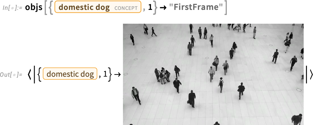
And, yup, that’s what it thought was a dog:

Game Theory

“What about game theory?”, people have long asked. And, yes, there has been lots of game theory done with the Wolfram Language, and lots of packages written for particular aspects of it. But in Version 14.2 we’re finally introducing built-in system functions for doing game theory (both matrix games and tree games).

Here’s how we specify a (zero-sum) 2-player matrix game:

This defines payoffs when each player takes each action. We can represent this by a dataset:

An alternative is to “plot the game” using MatrixGamePlot:

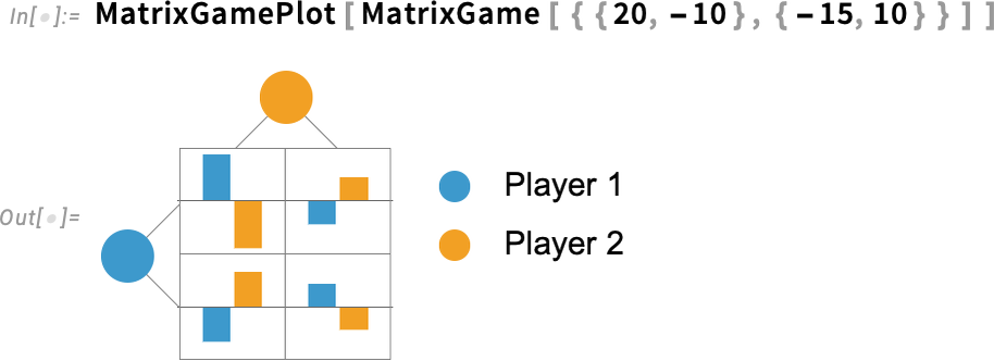
OK, so how can we “solve” this game? In other words, what action should each player take, with what probability, to maximize their average payoff over many instances of the game? (It’s assumed that in each instance the players simultaneously and independently choose their actions.) A “solution” that maximizes expected payoffs for all players is called a Nash equilibrium. (As a small footnote to history, John Nash was a long-time user of Mathematica and what’s now the Wolfram Language—though many years after he came up with the concept of Nash equilibrium.) Well, now in Version 14.2, FindMatrixGameStrategies computes optimal strategies (AKA Nash equilibria) for matrix games:

This result means that for this game player 1 should play action 1 with probability and action 2 with probability , and player 2 should do these with probabilities and . But what are their expected payoffs? MatrixGamePayoff computes that:

It can get pretty hard to keep track of the different cases in a game, so MatrixGame lets you give whatever labels you want for players and actions:

These labels are then used in visualizations:

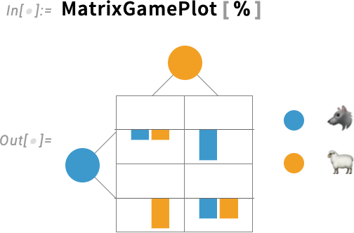
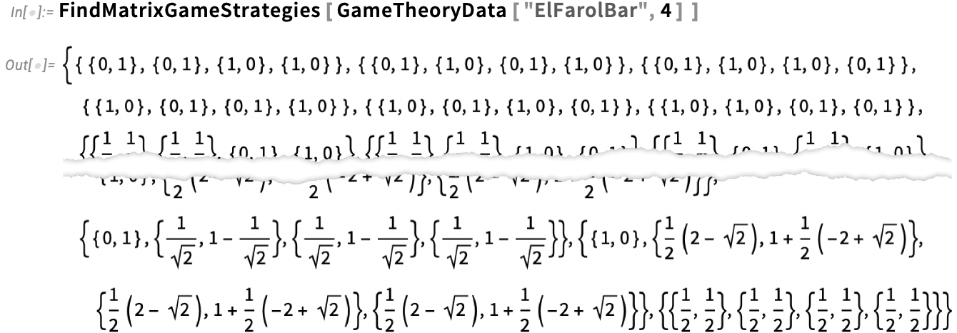
What we just showed is actually a standard example game—the “prisoner’s dilemma”. In the Wolfram Language we now have GameTheoryData as a repository of about 50 standard games. Here’s one, specified to have 4 players:

And it’s less trivial to solve this game, but here’s the result—with 27 distinct solutions:

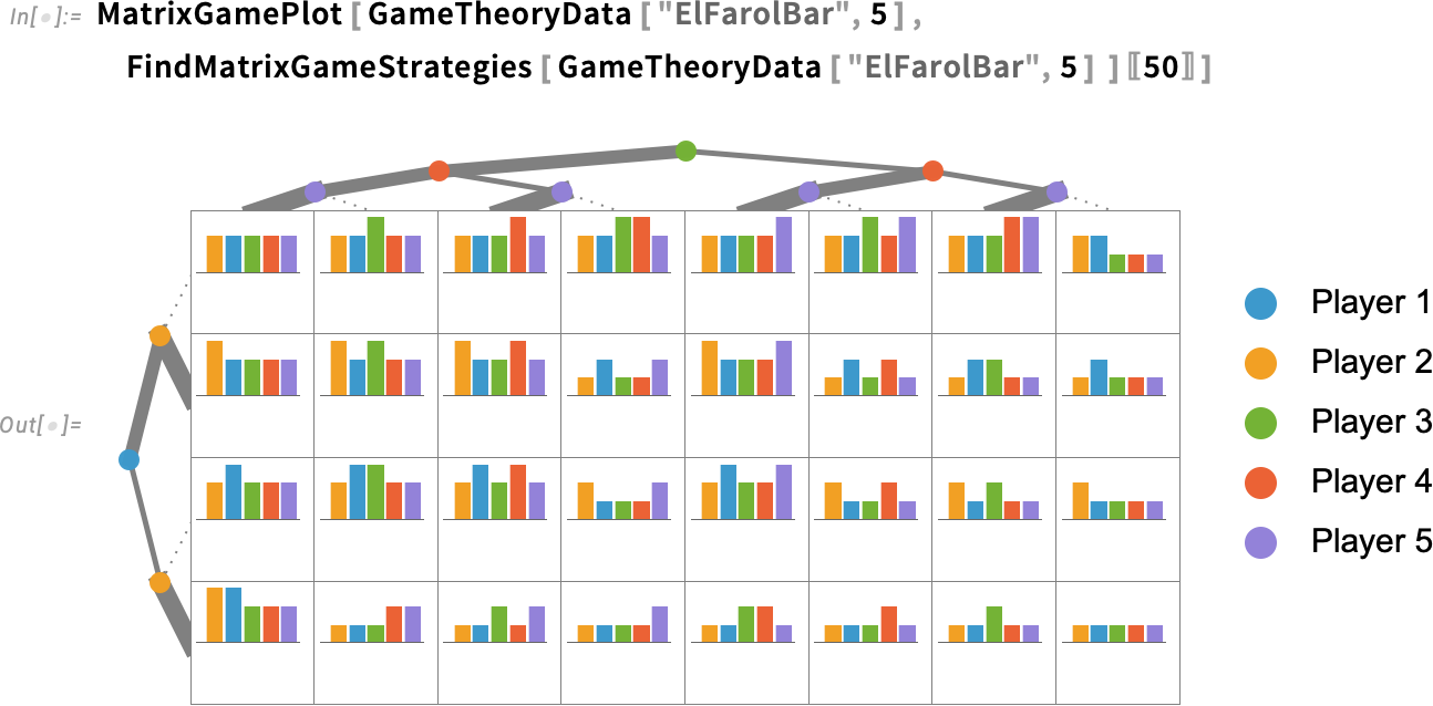
And, yes, the visualizations keep on working, even when there are more players (here we’re showing the 5-player case, indicating the 50th game solution):

It might be worth mentioning that the way we’re solving these kinds of games is by using our latest polynomial equation solving capabilities—and not only are we able to routinely find all possible Nash equilibria (not just a single fixed point), but we’re also able to get exact results:

In addition to matrix games, which model games in which players simultaneously pick their actions just once, we’re also supporting tree games, in which players take turns, producing a tree of possible outcomes, ending with a specified payoff for each of the players. Here’s an example of a very simple tree game:

We can get at least one solution to this game—described by a nested structure that gives the optimal probabilities for each action of each player at each turn:

Things with tree games can get more elaborate. Here’s an example—in which other players sometimes don’t know which branches were taken (as indicated by states joined by dashed lines):

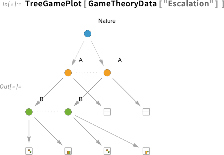
What we’ve got in Version 14.2 represents rather complete coverage of the basic concepts in a typical introductory game theory course. But now, in typical Wolfram Language fashion, it’s all computable and extensible—so you can study more realistic games, and quickly do lots of examples to build intuition.

We’ve so far concentrated on “classic game theory”, notably with the feature (relevant to many current applications) that all action nodes are the result of a different sequence of actions. However, games like tic-tac-toe (that I happened to recently study using multiway graphs) can be simplified by merging equivalent action nodes. Multiple sequences of actions may lead to the same game of tic-tac-toe, as is often the case for iterated games. These graph structures don’t fit into the kind of classic game theory trees we’ve introduced in Version 14.2—though (as my own efforts I think demonstrate) they’re uniquely amenable to analysis with the Wolfram Language.

Computing the Syzygies, and Other Advances in Astronomy

There are lots of “coincidences” in astronomy—situations where things line up in a particular way. Eclipses are one example. But there are many more. And in Version 14.2 there’s now a general function FindAstroEvent for finding these “coincidences”, technically called syzygies (“sizz-ee-gees”), as well as other “special configurations” of astronomical objects.

A simple example is the September (autumnal) equinox:

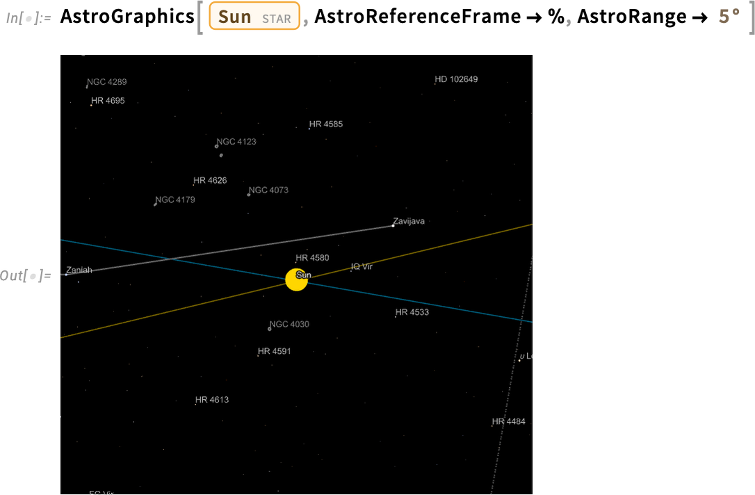
Roughly this is when day and night are of equal length. More precisely, it’s when the sun is at one of the two positions in the sky where the plane of the ecliptic (i.e. the orbital plane of the earth around the sun) crosses the celestial equator (i.e. the projection of the earth’s equator)—as we can see here (the ecliptic is the yellow line; the celestial equator the blue one):

As another example, let’s find the next time over the next century when Jupiter and Saturn will be closest in the sky:

They’ll get close enough to see their moons together:

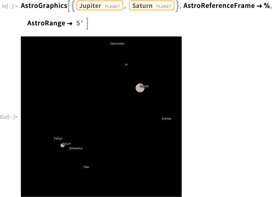
There are an incredible number of astronomical configurations that have historically been given special names. There are equinoxes, solstices, equiluxes, culminations, conjunctions, oppositions, quadratures—as well as periapses and apoapses (specialized to perigee, perihelion, periareion, perijove, perikrone, periuranion, periposeideum, etc.). In Version 14.2 we support all these.

So, for example, this gives the next time Triton will be closest to Neptune:

A famous example has to do with the perihelion (closest approach to the Sun) of Mercury. Let’s compute the position of Mercury (as seen from the Sun) at all its perihelia in the first couple of decades of the nineteenth century:

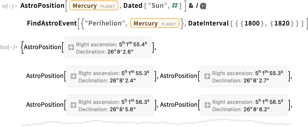
We see that there’s a systematic “advance” (along with some wiggling):

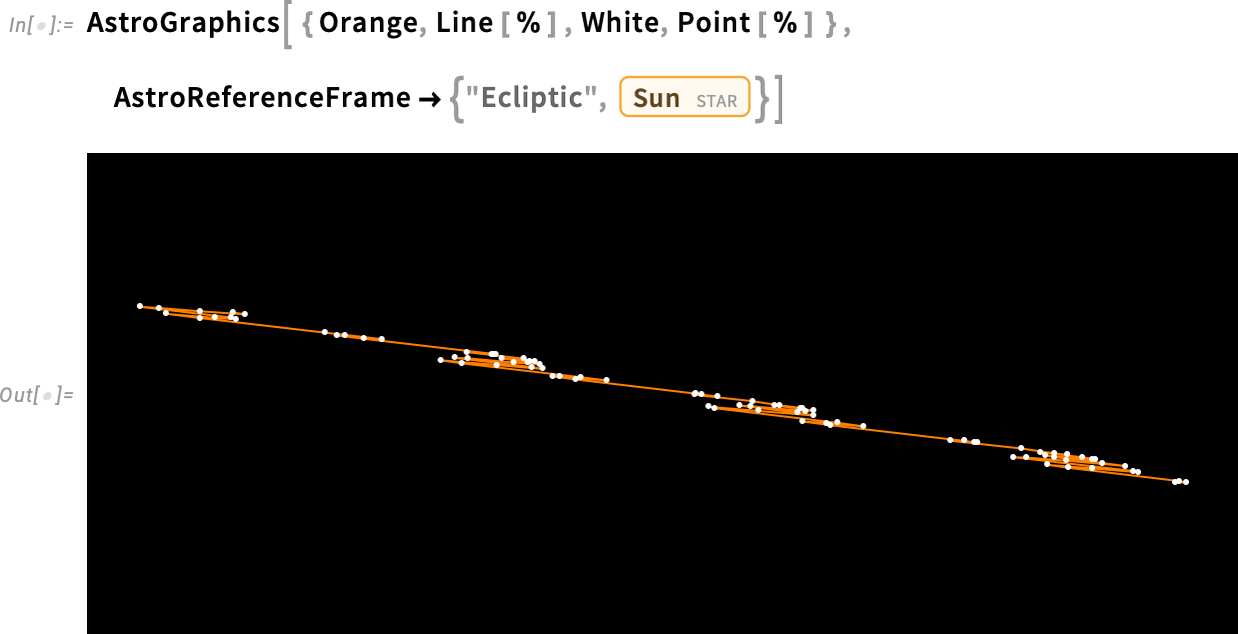
So now let’s quantitatively compute this advance. We start by finding the times for the first perihelia in 1800 and 1900:

Now we compute the angular separation between the positions of Mercury at these times:

Then divide this by the time difference

and convert units:

Famously, 43 arcseconds per century of this is the result of deviations from the inverse square law of gravity introduced by general relativity—and, of course, accounted for by our astronomical computation system. (The rest of the advance is the result of traditional gravitational effects from Venus, Jupiter, Earth, etc.)

PDEs Now Also for Magnetic Systems

More than a decade and a half ago we made the commitment to make the Wolfram Language a full strength PDE modeling environment. Of course it helped that we could rely on all the other capabilities of the Wolfram Language—and what we’ve been able to produce is immeasurably more valuable because of its synergy with the rest of the system. But over the years, with great effort, we’ve been steadily building up symbolic PDE modeling capabilities across all the standard domains. And at this point I think it’s fair to say that we can handle—at an industrial scale—a large part of the PDE modeling that arises in real-world situations.

But there are always more cases for which we can build in capabilities, and in Version 14.2 we’re adding built-in modeling primitives for static and quasistatic magnetic fields. So, for example, here’s how we can now model an hourglass-shaped magnet. This defines boundary conditions—then solves the equations for the magnetic scalar potential:

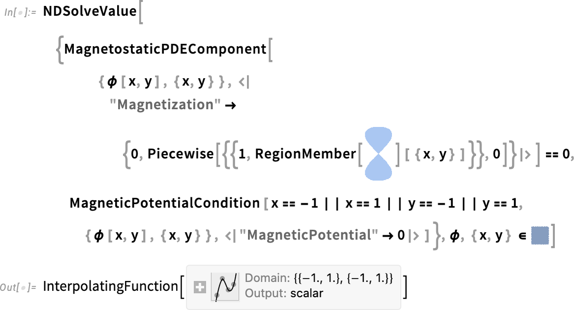
We can then take that result, and, for example, immediately plot the magnetic field lines it implies:

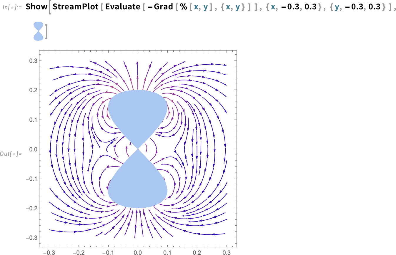
Version 14.2 also adds the primitives to deal with slowly varying electric currents, and the magnetic fields they generate. All of this immediately integrates with our other modeling domains like heat transfer, fluid dynamics, acoustics, etc.

There’s much to say about PDE modeling and its applications, and in Version 14.2 we’ve added more than 200 pages of additional textbook-style documentation about PDE modeling, including some research-level examples.

New Features in Graphics, Geometry & Graphs

Graphics has always been a strong area for the Wolfram Language, and over the past decade we’ve also built up very strong computational geometry capabilities. Version 14.2 adds some more “icing on the cake”, particularly in connecting graphics to geometry, and connecting geometry to other parts of the system.

As an example, Version 14.2 adds geometry capabilities for more of what were previously just graphics primitives. For example, this is a geometric region formed by filling a Bezier curve:

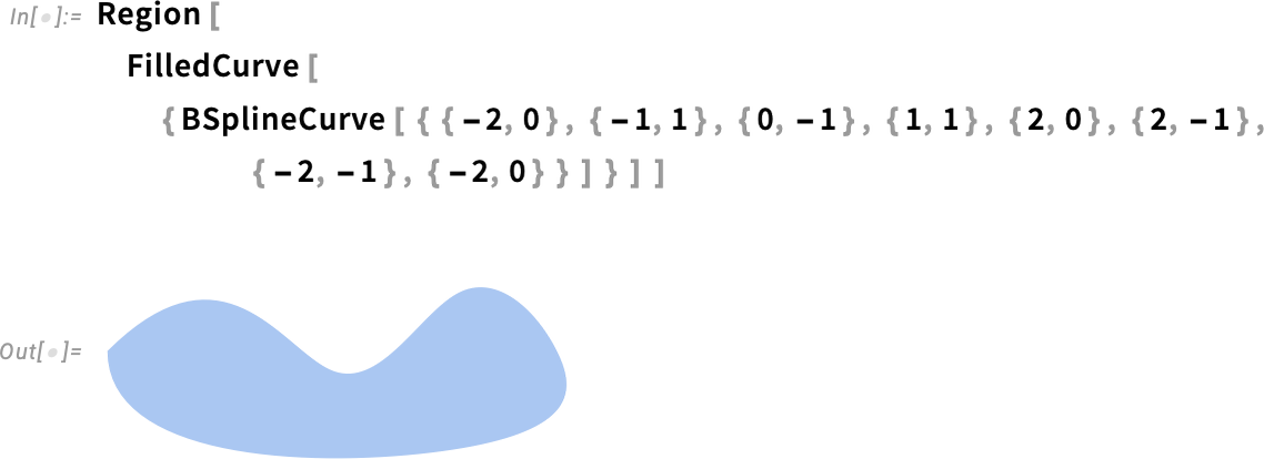
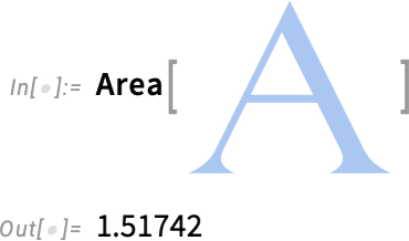
And we can now do all our usual computational geometry operations on it:

Something like this now works too:

Something else new in Version 14.2 is MoleculeMesh, which lets you build computable geometry from molecular structures. Here’s a graphical rendering of a molecule:

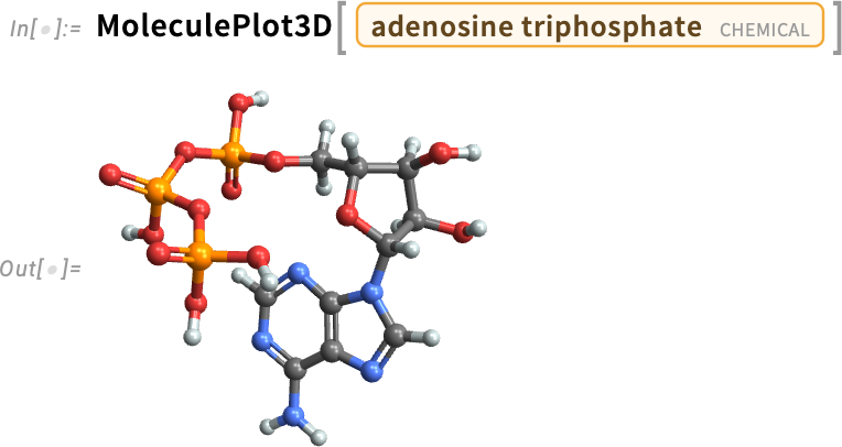
And here now is a geometric mesh corresponding to the molecule:

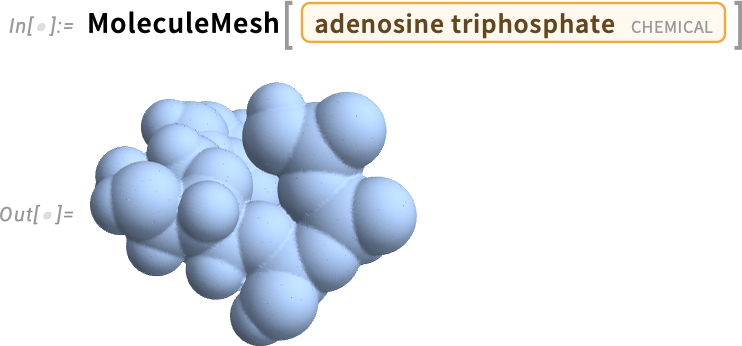
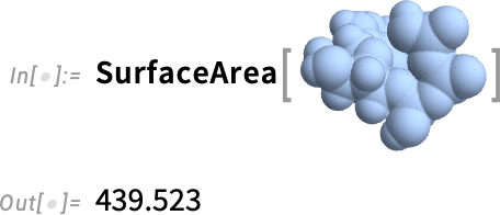
We can then do computational geometry on this mesh:

Another new feature in Version 14.2 is an additional method for graph drawing that can make use of symmetries. If you make a layered graph from a symmetrical grid, it won’t immediately render in a symmetrical way:

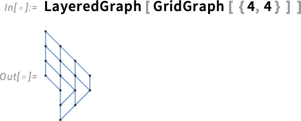
But with the new "SymmetricLayeredEmbedding" graph layout, it will:

User Interface Tune-Ups

Making a great user interface is always a story of continued polishing, and we’ve now been doing that for the notebook interface for nearly four decades. In Version 14.2 there are several notable pieces of polish that have been added. One concerns autocompletion for option values.

We’ve long shown completions for options that have a discrete collection of definite common settings (such as All, Automatic, etc.). In Version 14.2 we’re adding “template completions” that give the structure of settings, and then let you tab through to fill in particular values. In all these years, one of the places I pretty much always find myself going to in the documentation is the settings for FrameLabel. But now autocompletion immediately shows me the structure of these settings:

Also in autocompletion, we’ve added the capability to autocomplete context names, context aliases, and symbols that include contexts. And in all cases, the autocompletion is “fuzzy” in the sense that it’ll trigger not only on characters at the beginning of a name but on ones anywhere in the name—which means that you can just type characters in the name of a symbol, and relevant contexts will appear as autocompletions.

Another small convenience added in Version 14.2 is the ability to drag images from one notebook to any other notebook, or, for that matter, to any other application that can accept dragged images. It’s been possible to drag images from other applications into notebooks, but now you can do it the other way too.

Something else that’s for now specific to macOS is enhanced support for icon preview (as well as Quick Look). So now if you have a folder full of notebooks and you select Icon view, you’ll see a little representation of each notebook as an icon of its content:

Under the hood in Version 14.2 there are also some infrastructural developments that will enable significant new features in subsequent versions. Some of these involve generalized support for dark mode. (Yes, one might initially imagine that dark mode would somehow be trivial, but when you start thinking about all the graphics and interface elements that involve colors, it’s clear it’s not. Though, for example, after significant effort we did recently release dark mode for Wolfram|Alpha.)

So, for example, in Version 14.2 you’ll find the new symbol LightDarkSwitched, which is part of the mechanism for specifying styles that will automatically switch for light and dark modes. And, yes, there is a style option LightDark that will switch modes for notebooks—and which is at least experimentally supported.

Related to light/dark mode is also the notion of theme colors: colors that are defined symbolically and can be switched together. And, yes, there’s an experimental symbol ThemeColor related to these. But the full deployment of this whole mechanism won’t be there until the next version.

The Beginnings of Going Native on GPUs

Many important pieces of functionality inside the Wolfram Language automatically make use of GPUs when they are available. And already 15 years ago we introduced primitives for low-level GPU programming. But in Version 14.2 we’re beginning the process of making GPU capabilities more readily available as a way to optimize general Wolfram Language usage. The key new construct is GPUArray, which represents an array of data that will (if possible) be stored so as to be immediately and directly accessible to your GPU. (On some systems, it will be stored in separate “GPU memory”; on others, such as modern Macs, it will be stored in shared memory in such a way as to be directly accessible by the GPU.)

In Version 14.2 we’re supporting an initial set of operations that can be performed directly on GPU arrays. The operations available vary slightly from one type of GPU to another. Over time, we expect to use or create many additional GPU libraries that will extend the set of operations that can be performed on GPU arrays.

Here is a random ten-million-element vector stored as a GPU array:

The GPU on the Mac on which I am writing this supports the necessary operations to do this purely in its GPU, giving back a GPUArray result:

Here’s the timing:

And here’s the corresponding ordinary (CPU) result:

In this case, the GPUArray result is about a factor of 2 faster. What factor you get will vary with the operations you’re doing, and the particular hardware you’re using. So far, the largest factors I’ve seen are around 10x. But as we build more GPU libraries, I expect this to increase—particularly when what you’re doing involves a lot of compute “inside the GPU”, and not too much memory access.

By the way, if you sprinkle GPUArray in your code it’ll normally never affect the results you get—because operations always default to running on your CPU if they’re not supported on your GPU. (Usually GPUArray will make things faster, but if there are too many “GPU misses” then all the “attempts to move data” may actually slow things down.) It’s worth realizing, though, that GPU computation is still not at all well standardized or uniform. Sometimes there may only be support for vectors, sometimes also matrices—and there may be different data types with different numerical precision supported in different cases.

And Even More…

In addition to all the things we’ve discussed here so far, there are also a host of other “little” new features in Version 14.2. But even though they may be “little” compared to other things we’ve discussed, they’ll be big if you happen to need just that functionality.

For example, there’s MidDate—that computes the midpoint of dates:

And like almost everything involving dates, MidDate is full of subtleties. Here it’s computing the week 2/3 of the way through this year:

In math, functions like DSolve and SurfaceIntegrate can now deal with symbolic array variables:

SumConvergence now lets one specify the range of summation, and can give conditions that depend on it:

A little convenience that, yes, I asked for, is that DigitCount now lets you specify how many digits altogether you want to assume your number has, so that it appropriately counts leading 0s:

Talking of conveniences, for functions like MaximalBy and TakeLargest we added a new argument that says how to sort elements to determine “the largest”. Here’s the default numerical order

and here’s what happens if we use “symbolic order” instead:

There are always so many details to polish. Like in Version 14.2 there’s an update to MoonPhase and related functions, both new things to ask about, and new methods to compute them:

In another area, in addition to major new import/export formats (particularly to support Tabular) there’s an update to "Markdown" import that gives results in plaintext, and there’s an update to "PDF" import that gives a mixed list of text and images.

And there are lots of other things too, as you can find in the “Summary of New and Improved Features in 14.2”. By the way, it’s worth mentioning that if you’re looking at a particular documentation page for a function, you can always find out what’s new in this version just by pressing show changes: