The Basic Setup
Whether one’s dealing with biology, economics, politics or a host of other fields, it’s common to encounter situations that can be modeled as involving two agents that repeatedly compete with each other. One imagines that at each step each agent can take one of a certain set of actions, and that then—in a classic game theory way—each agent (or “player”) gets a certain fixed “payoff” based on the action they and their opponent take. But how do the agents decide what action to take? We imagine that each agent has a certain fixed procedure—or “strategy”—for making its decisions. And we imagine that the input to each of those decisions is the sequence of past actions that the agent and its opponent have taken.
There’s been lots of work done over the course of nearly a century on particular choices of strategies. But something I’ve long been curious about is what happens if one systematically considers all possible strategies. And if we think of strategies as programs this becomes a question to which we can immediately apply ruliological methods. Which is what I’m going to do here.
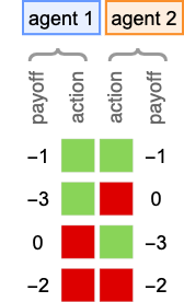
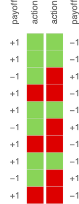
To be more specific about the setup, let’s assume that at each step, each agent takes one of two possible actions, indicated by ![]() and
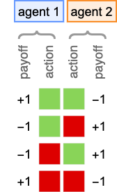
and ![]() . And for now let’s take the payoffs to be the ones for the classic “match-or-not” (“matching pennies”) game—in which player 1 has the bigger payoff when there’s a match, and player 2 has the bigger payoff when there isn’t a match:
. And for now let’s take the payoffs to be the ones for the classic “match-or-not” (“matching pennies”) game—in which player 1 has the bigger payoff when there’s a match, and player 2 has the bigger payoff when there isn’t a match:
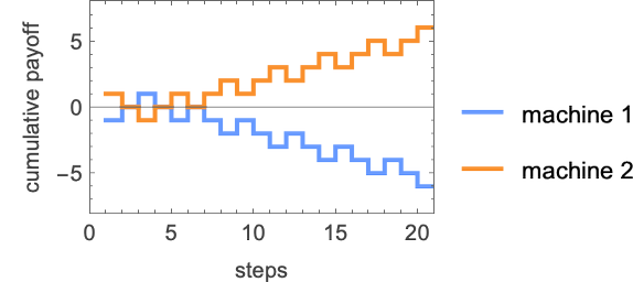
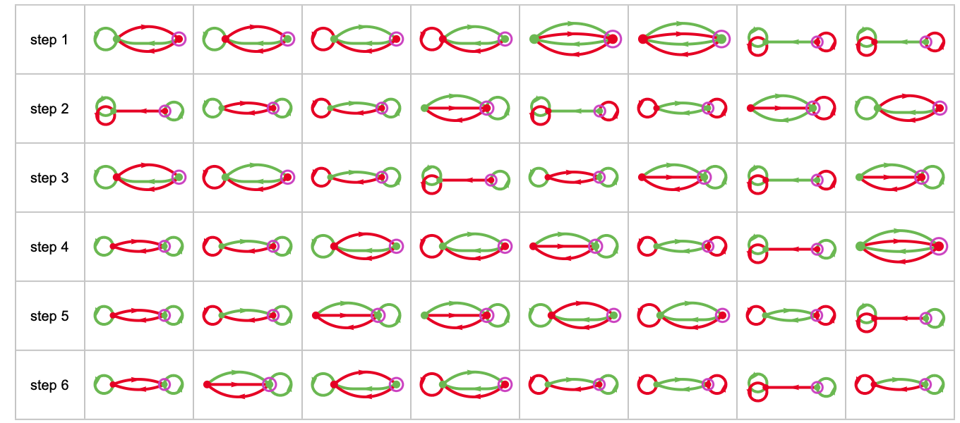
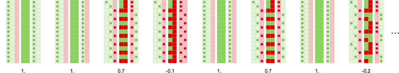
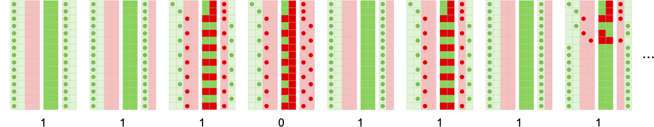
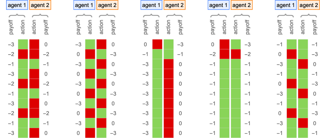
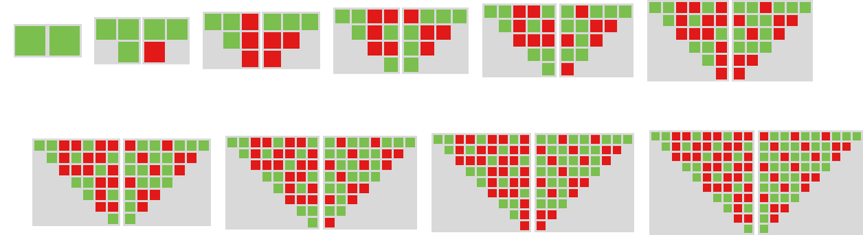
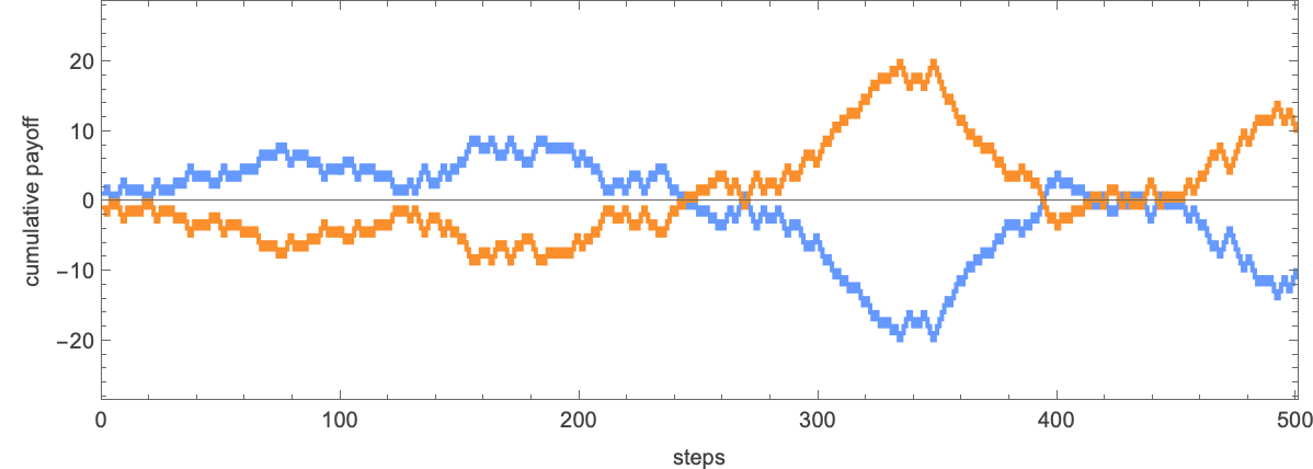
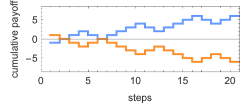
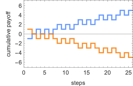
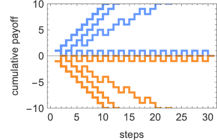
So what happens when agents repeatedly play this game? Well, it depends on their strategies. Here are a few examples for several different choices of each agent’s strategy:
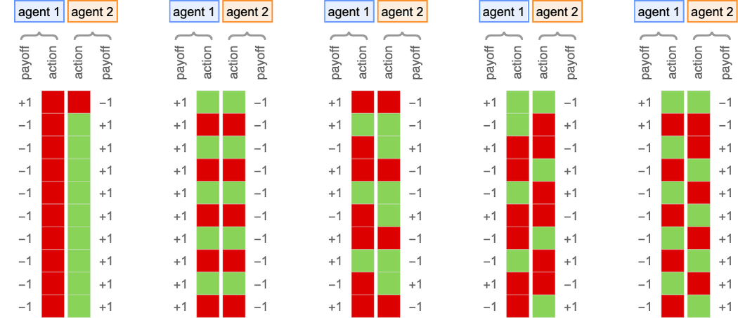
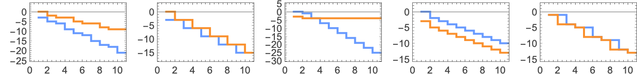
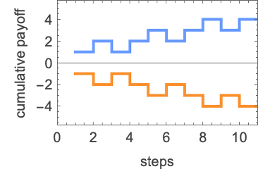
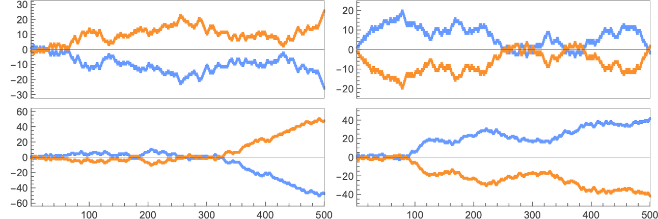
Plotting the cumulative payoffs for the two agents (represented by ![]() and
and ![]() ) in each of these cases we get:
) in each of these cases we get:
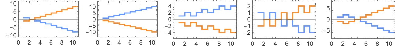
Often we’ll consider the “winning agent” to be the one that has the numerically largest cumulative payoff (i.e. is eventually on top in these plots) after a certain number of steps. And with a criterion like this, we’ll be able to rank different programs against each other—and in general explore the ruliology of competition.
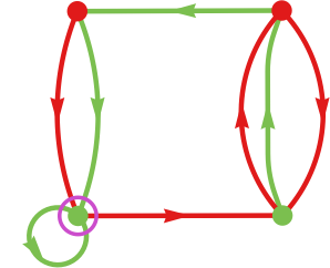
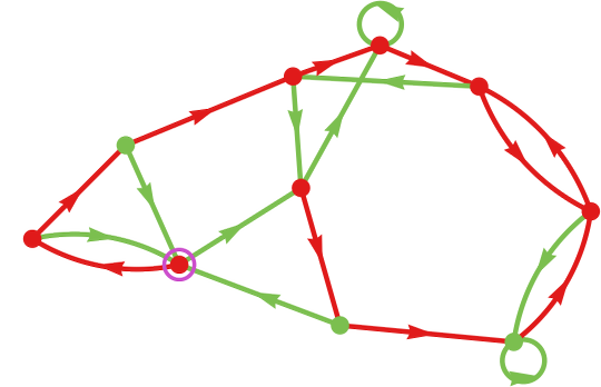
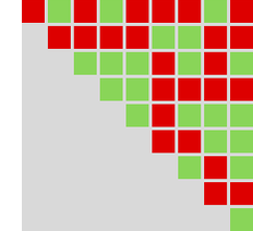
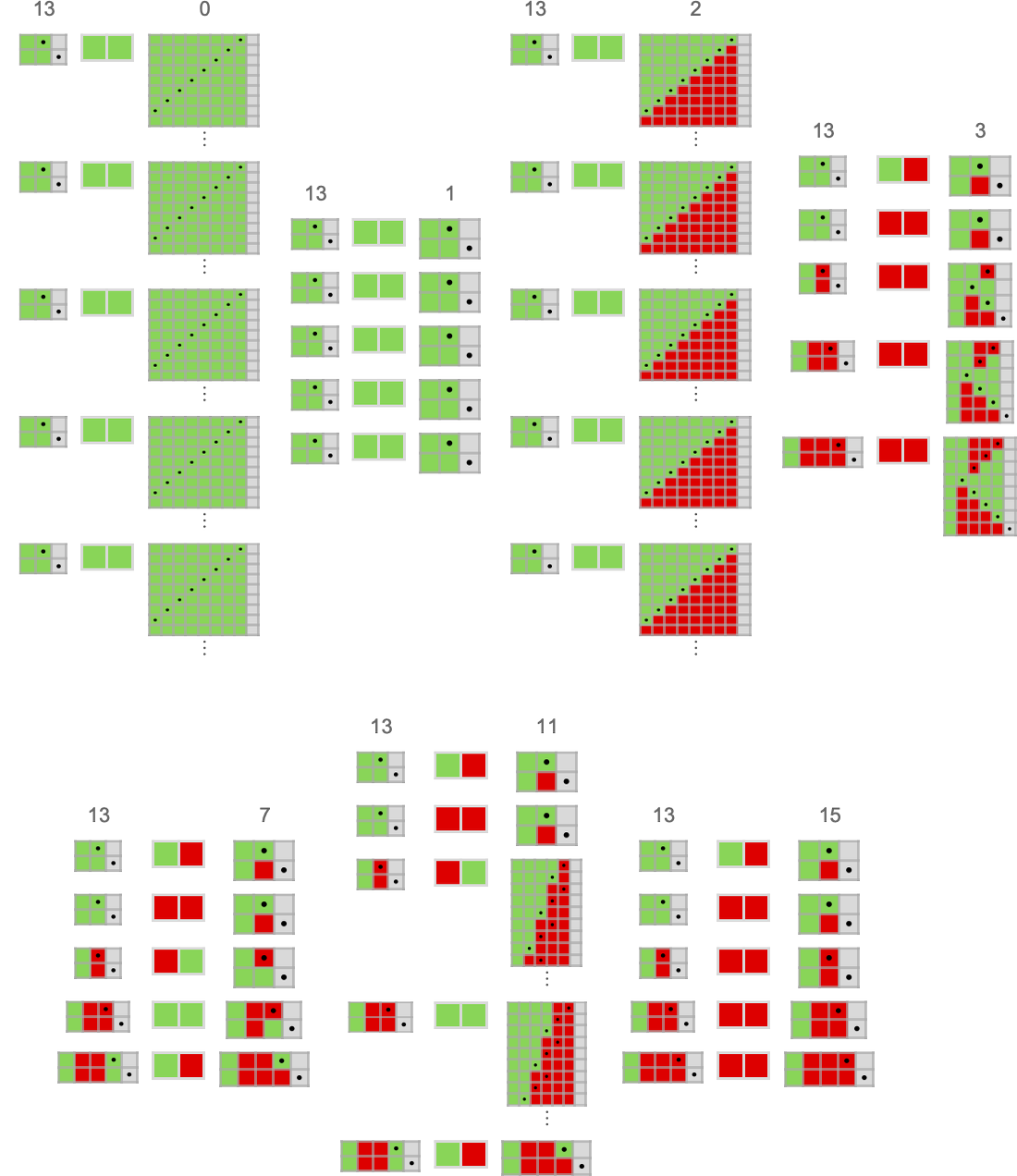
With the basic setup we’re using, we can represent all possible sequences of actions by a multiway graph:
For any given sequence of actions, there is then a cumulative payoff for each agent for our match-or-not game:
If each agent adopts a particular strategy, this will define a particular path through the multiway graph. For the strategies used in the examples above, the paths are:
What does it take to have a winning strategy? In what follows, we’ll consider strategies based on several different types of programs. But one basic question we can always ask is whether what turn out to be the winning strategies tend to be based on programs that are more complicated, or less so—or to show behavior that is more complicated, or less so.
In other words, if you want to win, should you typically be trying to build up something complicated? Or should you instead expect to be able to find a “simple hack” that will “crack the game” and—at least usually—let you win? In effect, we’re asking whether competition tends to lead to complexity, or simplicity.
I’ve recently looked at minimal models of both biological evolution and machine learning, in which one is adaptively evolving programs in order to maximize some externally imposed fitness function. And what I’ve found is that even when the fitness function one uses is simple, the behavior of the programs that maximize it is normally quite complex. In other words, adaptive evolution will tend to make even a simple, fixed objective be achieved in a complicated way.
So what if instead of having a fixed, externally imposed objective, our goal is just broadly to win against other agents? Does such—potentially open-ended—competition lead us to more complex behavior (or more complex programs), or not? That’s the kind of question we’re going to be able to explore here by looking at the ruliology of competition.
Strategies from Finite State Machines
Finite state machines can be thought of as defining extremely simple programs (that might model pathways in biology, decision processes in economics, etc.). And to start our investigation of the ruliology of competition we’re going to look at strategies defined by finite state machines.
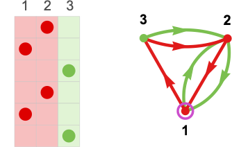
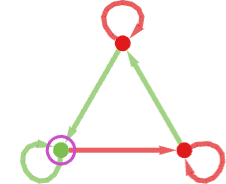
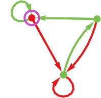
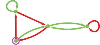
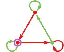
A typical example of a finite state machine (here with 3 states) is:
We’re going to use this finite state machine to define a strategy for an agent. To see how this works, let’s say that the sequence of actions taken by the agent’s opponent have been:
The idea is to use this sequence of actions to define a path in the finite-state-machine graph, then to determine the next action from the color of the state reached. We start at the vertex with the incoming arrow, then successively follow the edge whose color matches the next move made by the opponent:
At the end of this process we’ll reach some vertex in the graph (i.e. some state in the finite state machine). In the particular case shown here, the state we reach is ![]() . And then we take the output of the strategy—i.e. the next action for the agent to take—to be
. And then we take the output of the strategy—i.e. the next action for the agent to take—to be ![]() .
.
It’s sometimes convenient to show the states of the finite state machine arranged on a line:
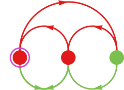
And then we can summarize the path taken with a certain input by showing the successive states reached:
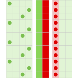
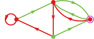
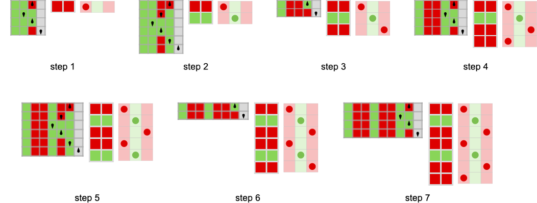
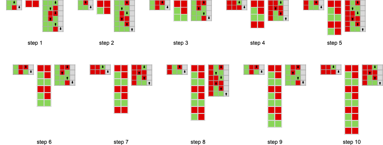
So what happens if two finite state machines compete? The basic idea is that the successive outputs from one machine become the successive inputs to the other, and vice versa. If our second machine is
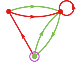
then we can represent the behavior of the machines by:
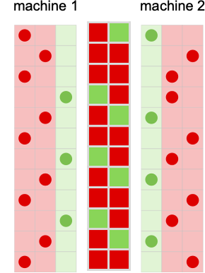
If the payoffs we use are for the match-or-not game, then their cumulative values for these machines are
so that in the end agent 2 can be considered the winner.
It’s important to note here that in the setup we’re using, everything is deterministic: at every step, each agent takes an action that is deterministically computed using its strategy from the past history of moves. It’s a different setup from what’s most often studied in game theory, where each move is in effect considered independently, but where there can be probabilities for different actions (“mixed strategies”)—and where in the end averaging is done over “different possible rolls of the dice”.
The Space of Possible Finite State Machines
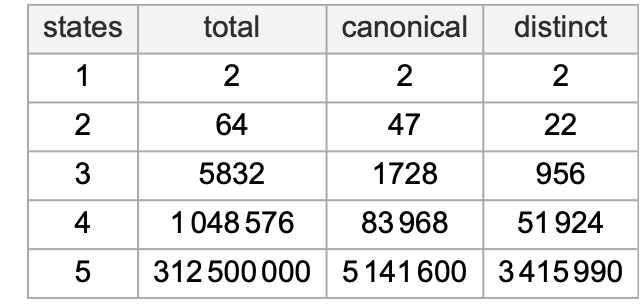
The number of possible graphs for finite state machines with s states is (2 s2)s. But some of those graphs correspond to machines with identical behavior—so that the number of distinct machines is smaller:
2-State Machines
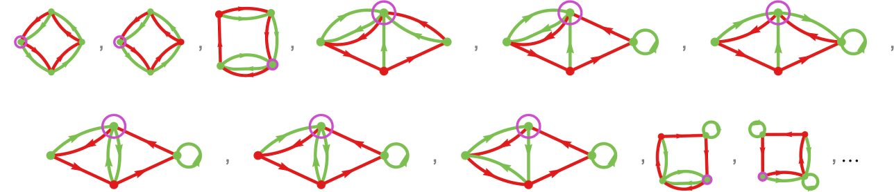
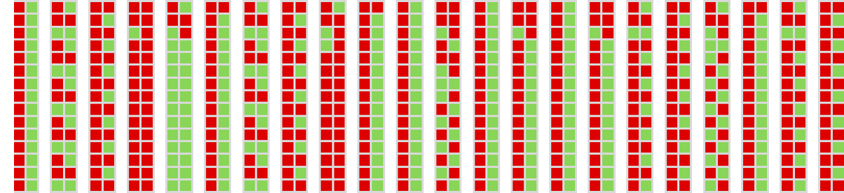
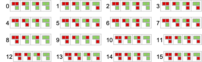
In the 2-state case, the 22 distinct machines are
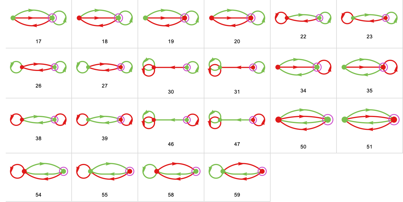
where we’ve identified each machine by a number.
So what happens if pairs of these machines compete? Here are a few examples, where in each case we’re identifying the average payoff (here for 10 rounds of the match-or-not game):
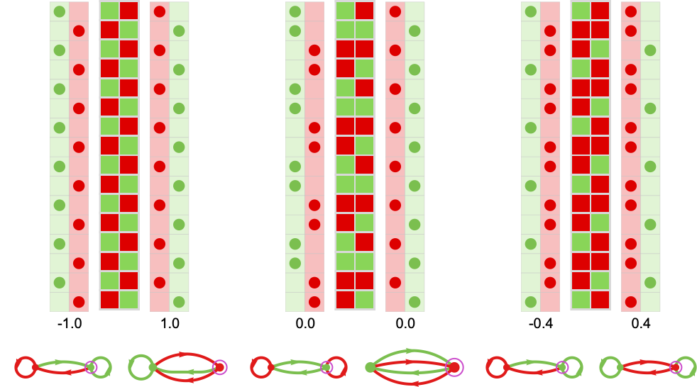
(In all competitions between pairs of finite state machines, the sequence of moves ultimately has to become periodic—with a period equal at most to the product of the number of states in each machine.)
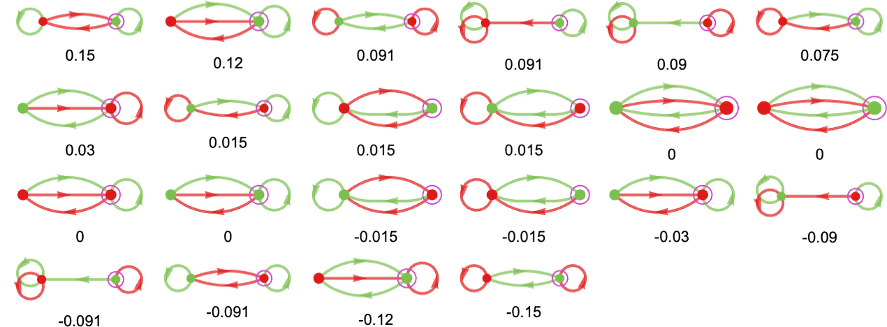
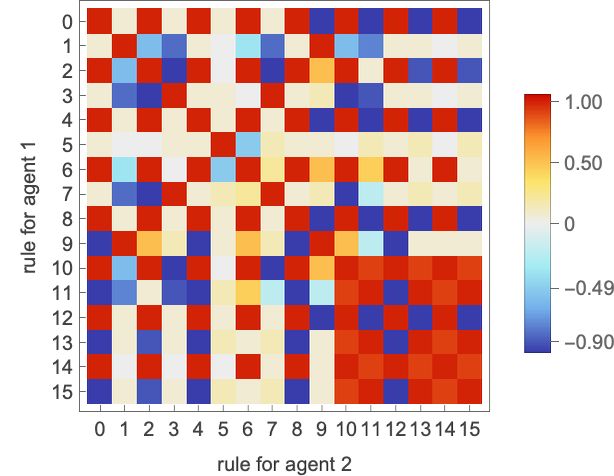
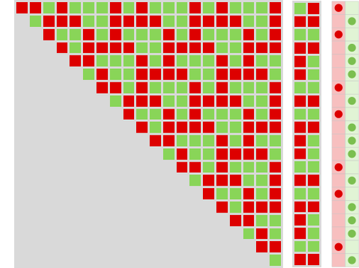
What happens if each of the 22 distinct 2-state machines competes against each of the other ones? We can summarize the results by showing the mean (long-term) payoff for every pair of machines (the payoff is for each machine “playing as agent 1”; in match-or-not, the payoff is negated if “playing as agent 2”):
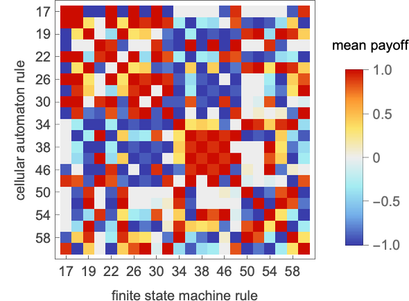
So what machine is the “overall winner”? One way to assess this is to look at the average of the mean payoffs achieved by a given machine when competing with all other (distinct) machines:
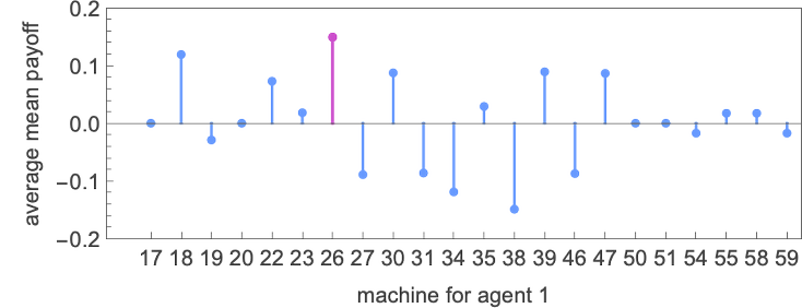
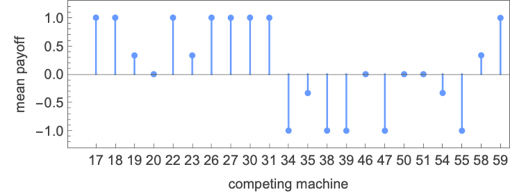
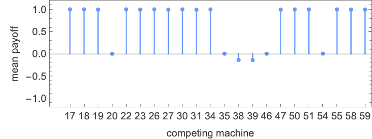
The winner by this measure is then machine 26:
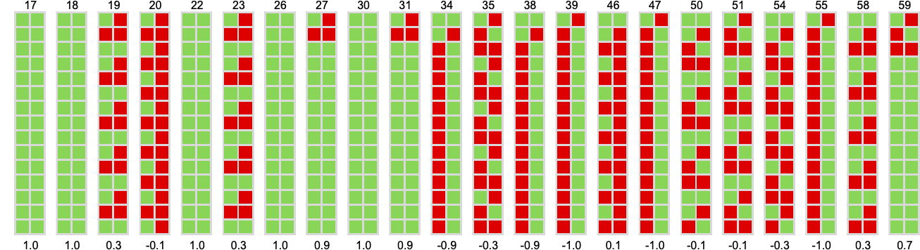
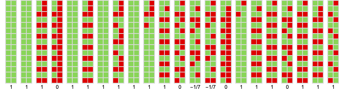
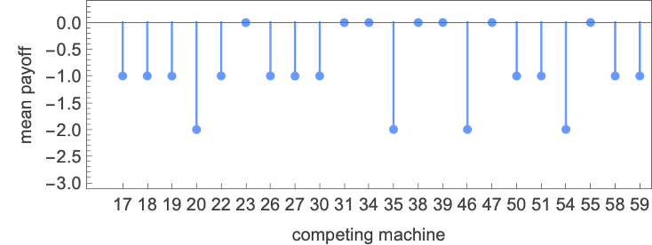
Running this machine against all (distinct) 2-state machines we get the following mean payoffs:
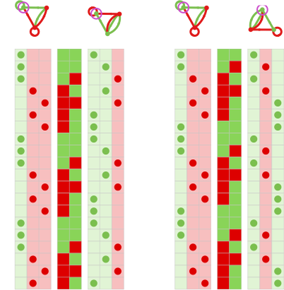
The actual behavior in each case—which doesn’t itself depend on the payoffs, only on the machines involved—is:
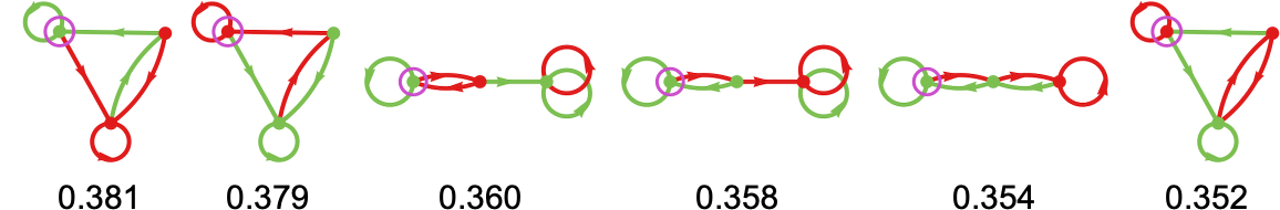
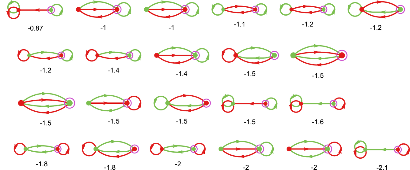
What are the “runners-up” to the winning machine? Here are all the distinct machines, ranked by their mean payoffs:
Here’s what happens if we play the top 3 runners-up against all machines:
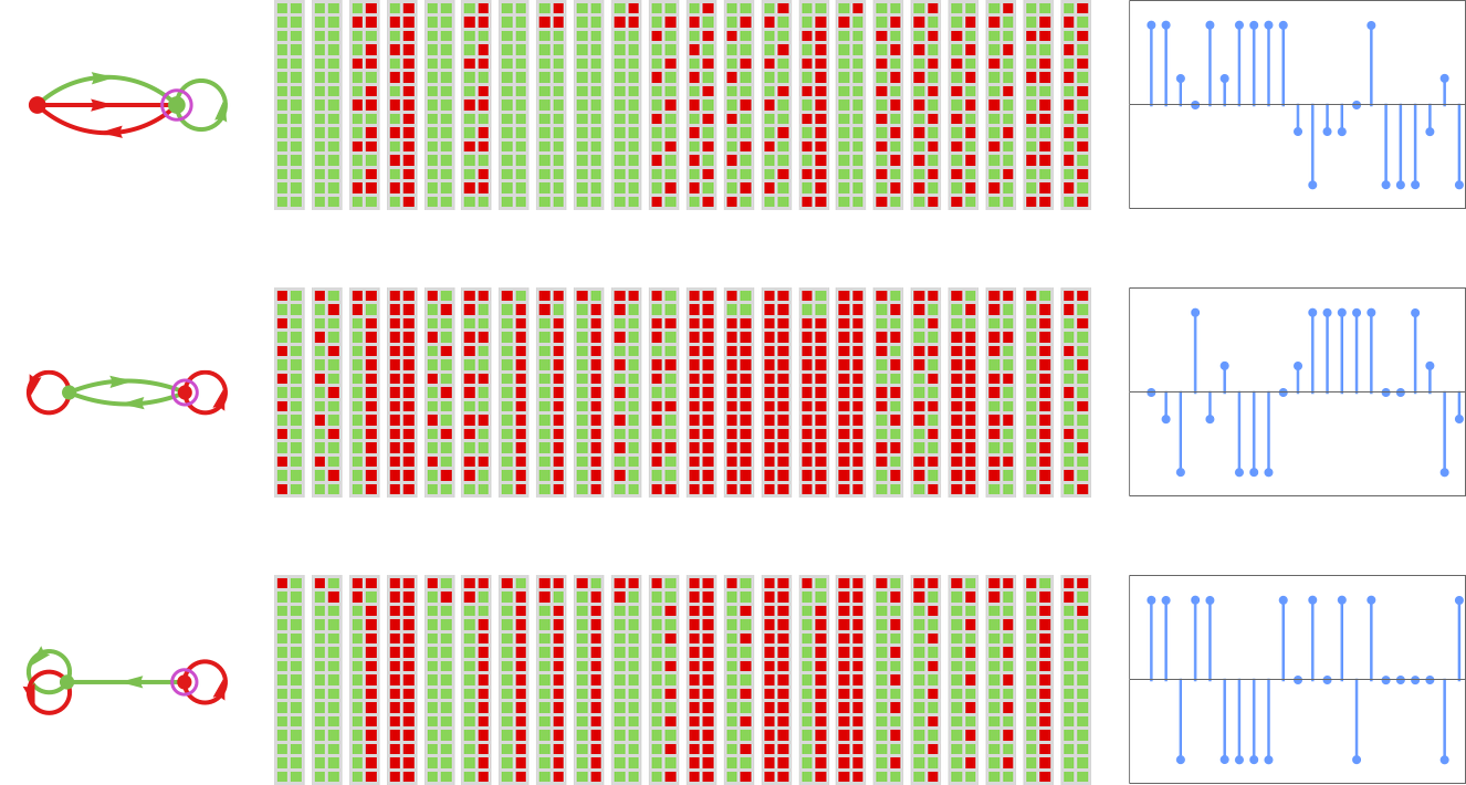
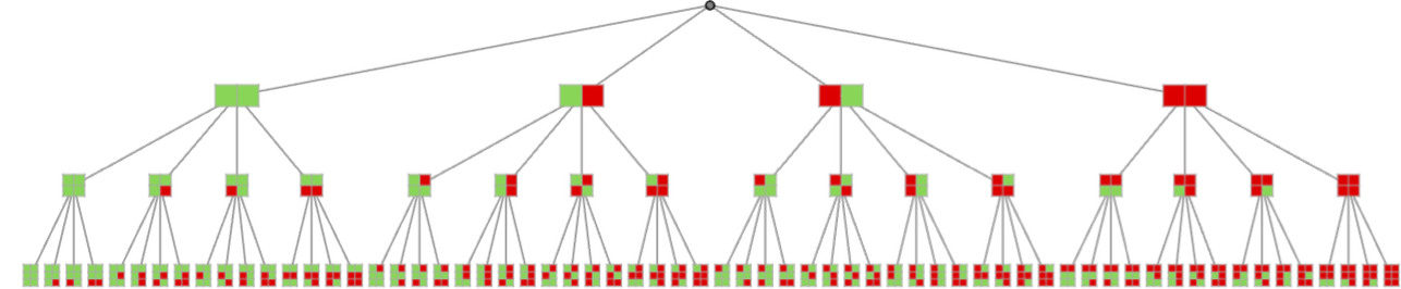
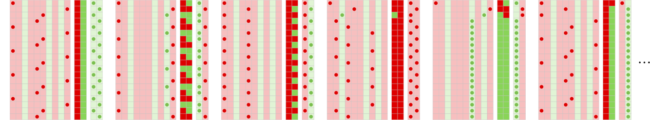
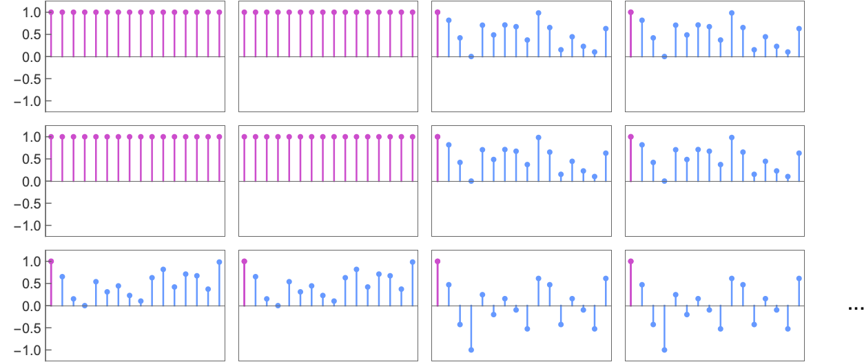
We can summarize how a machine behaves by showing the history of its behavior when playing against all other machines (or, in effect, by putting together the first columns in pictures like the ones above). Here are the results for all the machines (for 15 steps), ordered from highest average score down:
(Once again, these pictures are completely determined just from the machines involved; the payoffs in the match-or-not game determine only their ordering.)
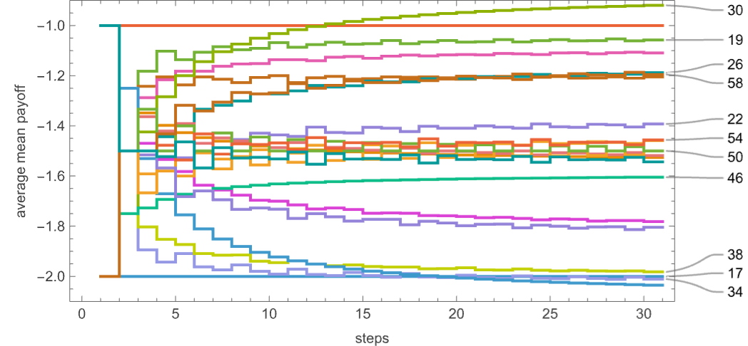
One footnote to what we’ve been saying here has to do with how many steps of competition we are getting the machines to do. For all finite-state machines, the behavior must eventually become periodic—and for 2-state machines the maximum period is 4 steps, with a maximum transient of 3 steps. But the actual average mean payoffs vary with the total number of steps one considers:
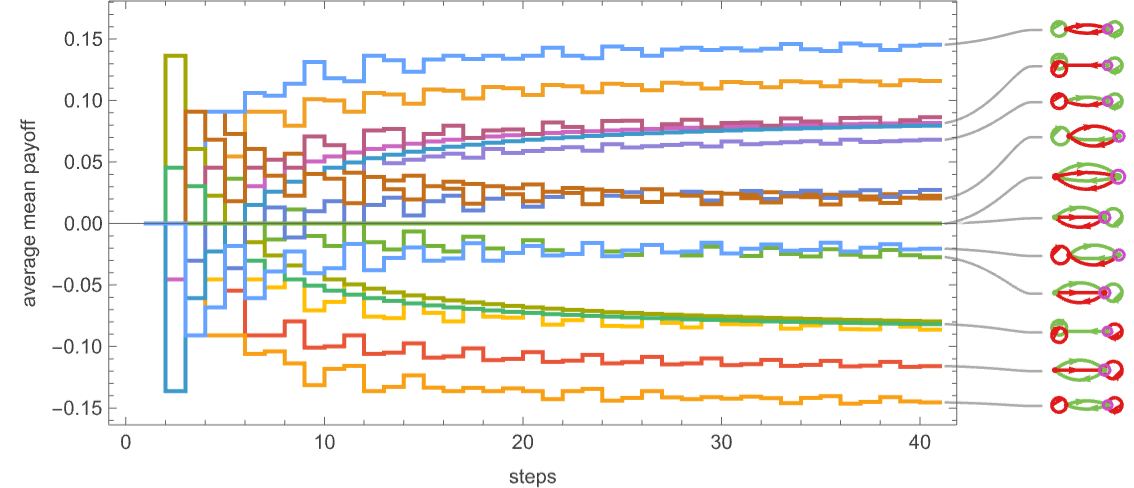
It’s notable that at the least for the first few steps, the rankings move around:
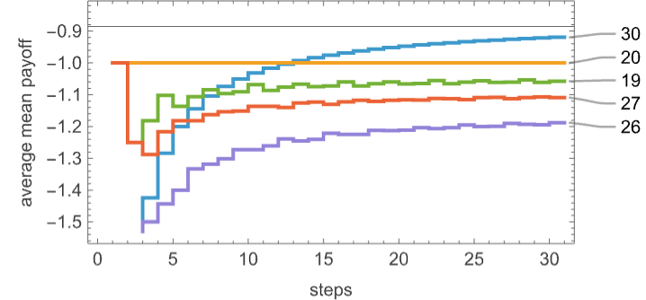
But in this case it doesn’t take too many steps for the ultimate winner to be clear (later on we’ll see examples where it takes much longer).
(There are other subtleties as well. One of them is that we are computing average payoffs by playing every machine against every other distinct machine. In principle we could also include other equivalent machines—which would slightly change the weighting of our averages. But since we’re really concerned with strategies, not machines as such, the scheme we’re using seems more appropriate.)
3-State Machines
For the 956 distinct machines with s = 3 states, the corresponding “competitive array” (after 1000 steps) is:
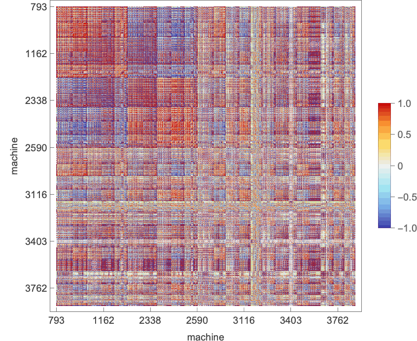
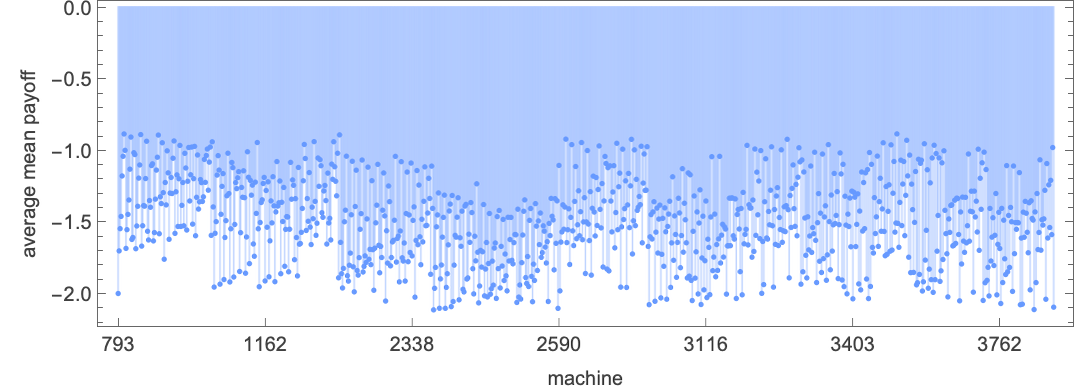
The average mean payoff for each of the machines (i.e. the average across each row in the “competitive array”) is then
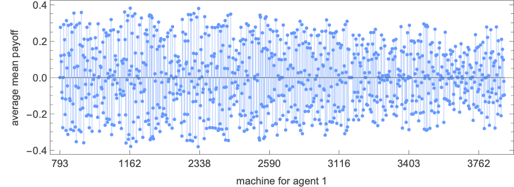
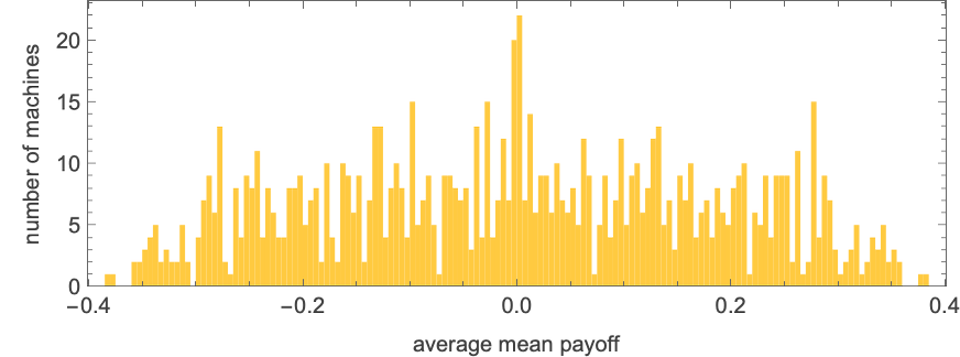
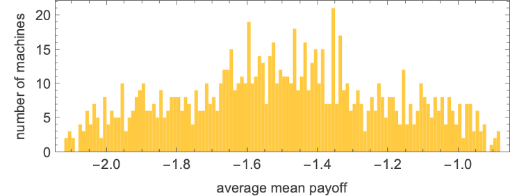
while the distribution of these average mean payoffs is:
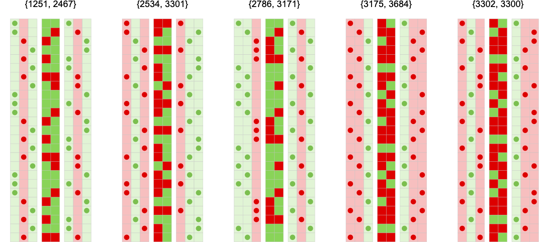
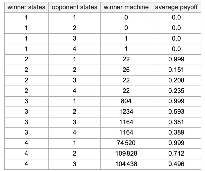
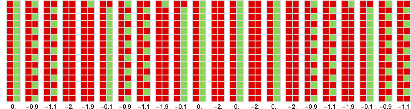
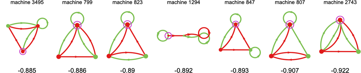
The top few machines for the match-or-not game are then:
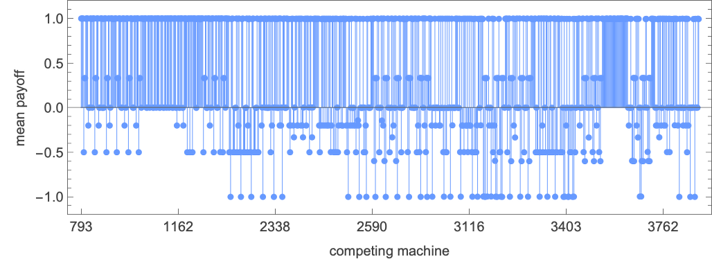
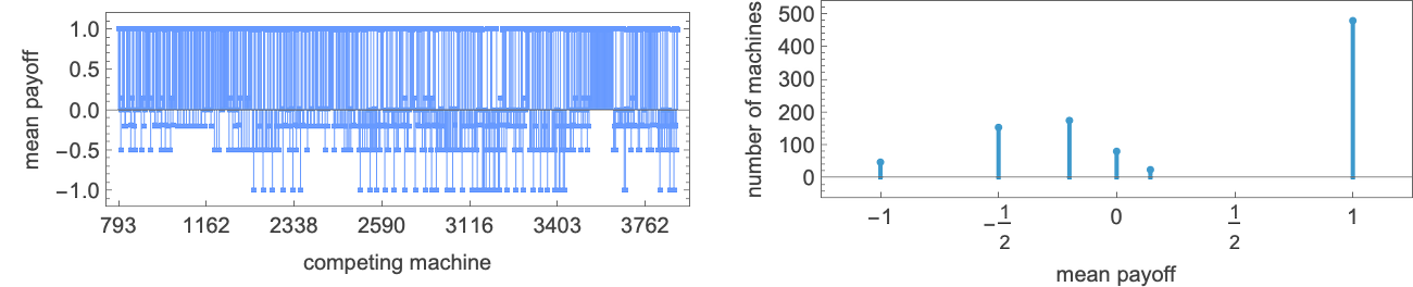
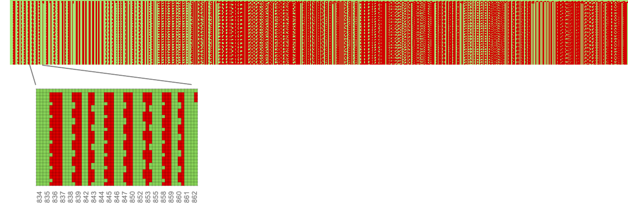
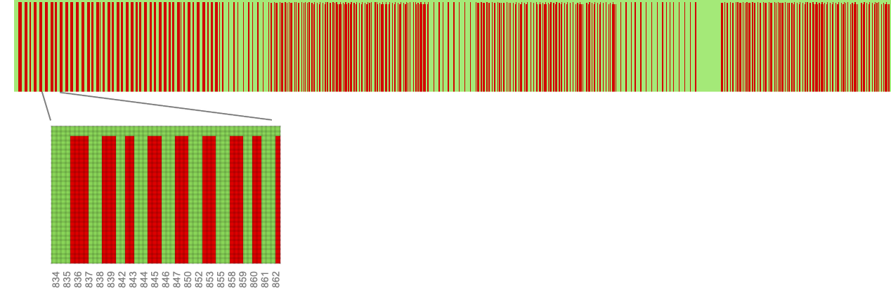
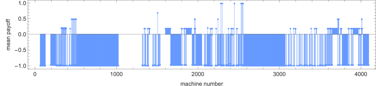
Running the top machine (s = 3 machine 1164) against all (distinct) 3-state machines we get the following mean payoffs:
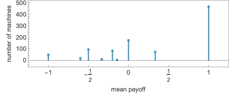
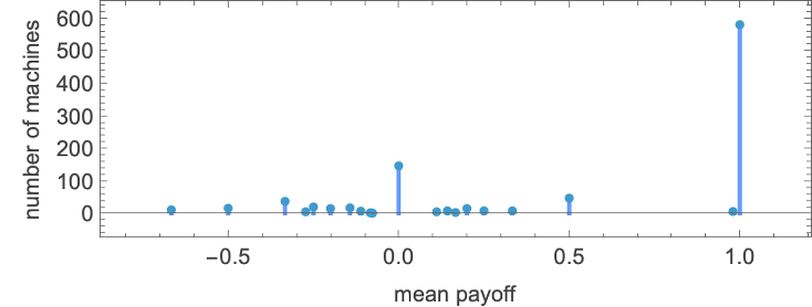
The distribution of possible limiting mean payoffs here is:
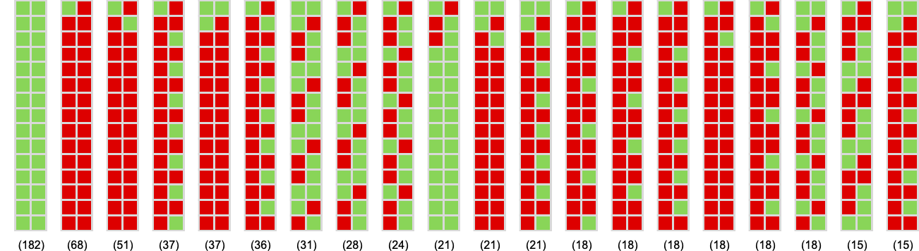
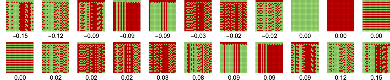
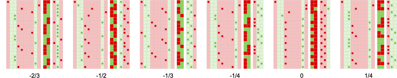
And the most common forms of behavior seen are:
The maximum possible period for a competition between two 3-state machines is 9. Machine 1164 never quite achieves this; its maximum period of 7 occurs when competing with machines 2546 and 2755 (both giving limiting mean payoff –1):
If one looks at all possible pairs of 3-state machines, there turn out to be 792 that yield period-9 behavior, examples being:
(These have no transients; the maximum transient for 3-state machines turns out to be 8.)
An Aside: What Do We Mean by “Average”?
We’ve talked about how a machine does “on average” when competing with all other (distinct) machines. But what do we mean by “on average”? So far, we’ve taken the “average” to be the mean of the payoffs obtained by competing with each other machine (and the payoffs here are themselves means across successive steps). But what if we use the median instead of the mean? Here are the median payoffs from running each machine for 1000 steps against all other machines:
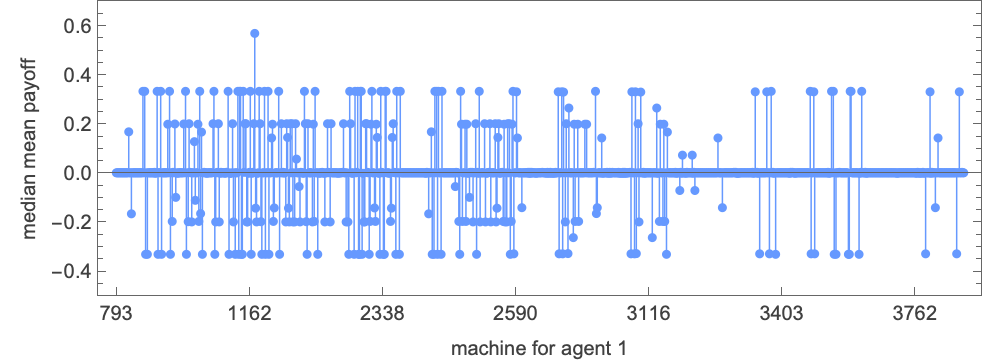
The standout winning machine here is machine 1172:
The mean payoffs and their distributions in this case are:
And the median is “anomalously high” because with this machine exactly 1/2 of all mean payoffs are +1. (The corresponding mean is pulled down by the “left tail” in the distribution of mean payoffs.)
The Complexity of Winning
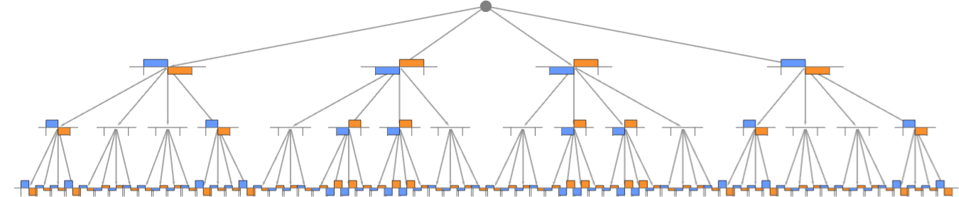
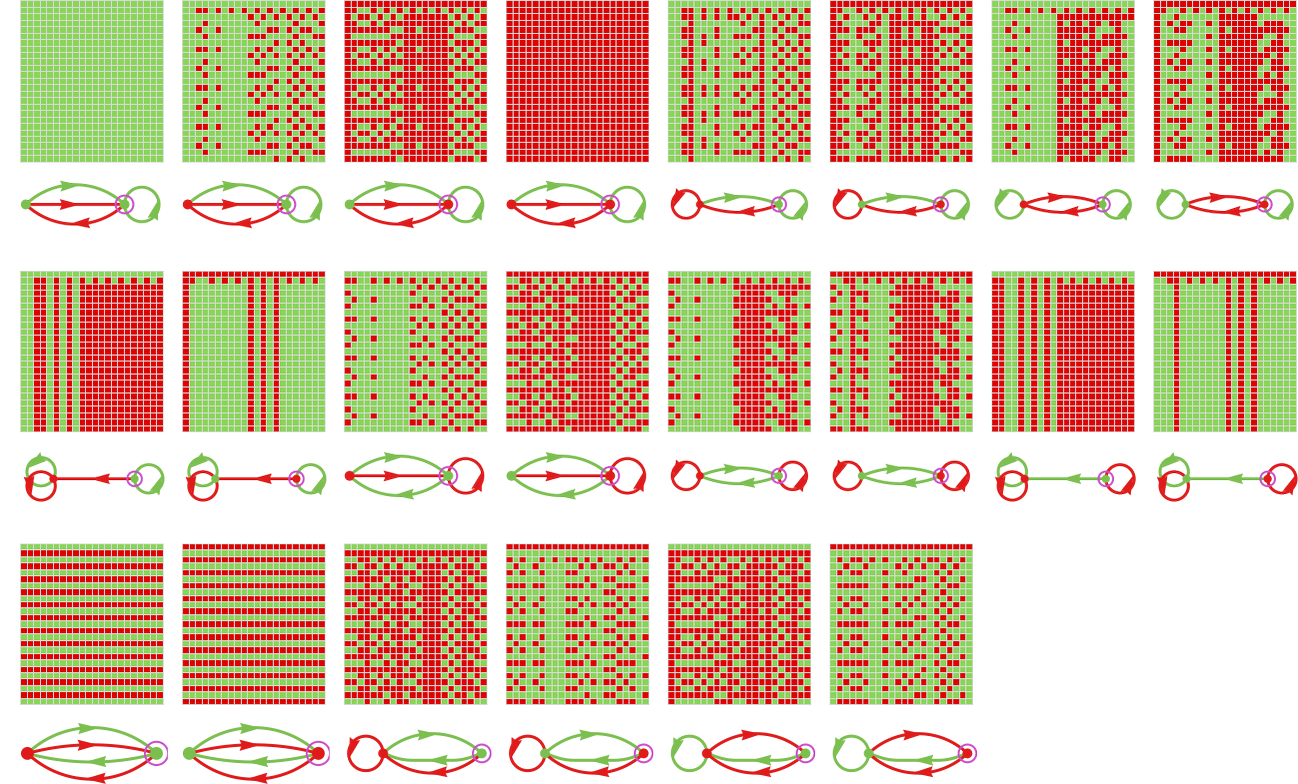
Let’s look (basically as above) at the actual behavior of each of the distinct 2-state finite state machines when competing against all other 2-state machines, ordered from smallest average mean payoff to largest:
The cases with 0 average mean payoff look simple in their behavior. But for other average mean payoffs, the behavior of a given machine competing against all others seems more complicated.
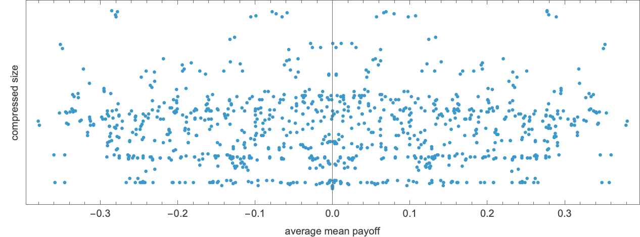
We can get some sense of this complexity by looking at the compressed size (as obtained from Compress) of the array of behavior shown above:
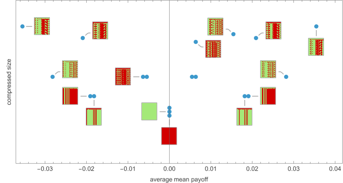
Here’s the corresponding result for the 956 distinct 3-state machines—showing no strong correlation between average mean payoff and our estimate of the complexity of behavior:
And indeed among machines with the highest average mean payoffs there is still quite a diversity of levels of complexity in behavior
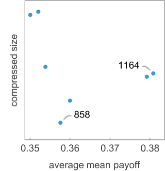
with the “behavior traces” of the machines indicated being
and
In other words, at least in this case, we really can’t say that winning machines are characterized either by being particularly complex in their behavior, or particularly simple. It seems that it’s detailed structure, rather than overall features, that determines what machines will win.
Competitions between Machines of Different Sizes
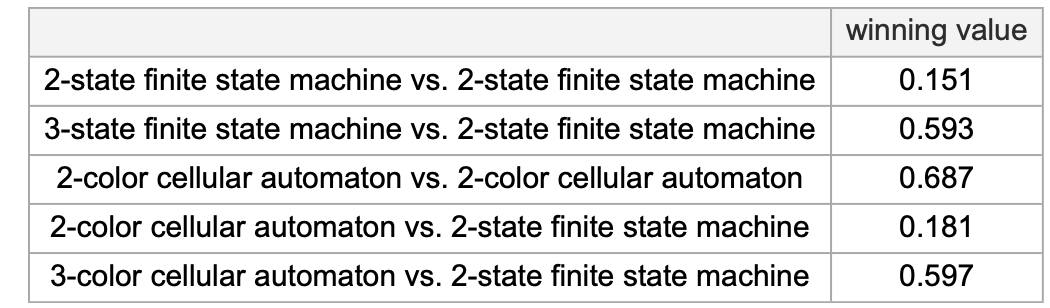
Can finite state machines with more states systematically do better (i.e. achieve larger payoffs) than ones with fewer states? The best average mean payoff any 2-state machine can achieve when competing with all other 2-state machines is about 0.151. But if, for example, we consider 3-state machines competing (for 1000 rounds) against 2-state machines, the best average mean payoff is instead 0.593:
Looking at the distribution of possible average mean payoffs, we see that the distribution of average mean payoffs is wider for 3-state machines than for 2-state ones—a fact that is at least partly just a consequence of there being many more possible 3-state machines than 2-state ones:
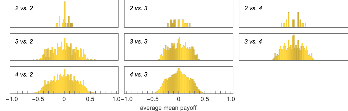
But something that’s notable is that the very broadest distribution is for 3-state machines competing against 2-state ones: in effect it seems that with their larger collection of possible strategies, the 3-state machines can do better at “outmaneuvering” the 2-state ones.
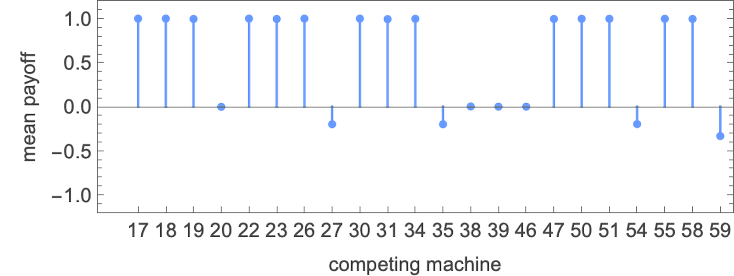
The 3-state machine that does the best overall against 2-state machines is machine 1234:
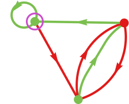
It doesn’t always definitively win (with mean payoff +1), but does so the majority of the time:
How does it achieve this? Basically, for lots of different 2-state machines, this particular 3-state machine manages to behave just as they do:
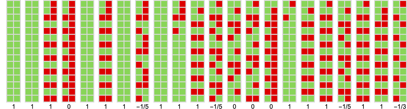
In some sense, there are facets of the 3-state machine that “resonate” with many 2-state ones:
How about 4-state machines? The 4-state machine that does best overall against 2-state machines is machine 109828:
Out of the 22 2-state machines, it only gets less than payoff +1 in 6 cases:
Here’s the behavior for all 22 cases:
And once again we can think of the 4-state machine as successfully “covering” most of the 2-state behaviors:
Adaptive Evolution of Finite State Machines
In many practical situations where there’s competition, there’s a way for the agents that are competing to evolve. So can we make a minimal model of this using finite state machines?
In what we’ve done so far, we’ve always been looking at a space of all possible finite state machines. But what about sequences of machines found by adaptive evolution? Is there, for example, a way to adaptively evolve machines to do progressively better in competitions?
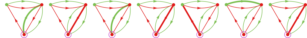
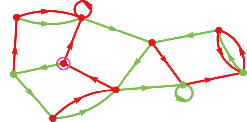
The first step in doing this is to see how we might make successive mutations to finite state machines. A simple approach is to say that any given mutation can affect either a random vertex or a random edge in the graph of a machine. For a vertex, the mutation just reverses its color. For an edge, it either reverses the color, or “reroutes” the edge to a different vertex (with the constraint that doing so doesn’t disconnect the graph). Applying a sequence of such mutations at random gives for example
or, with a different graph rendering:
(Note that we’re mutating machines in whatever form we find them; we’re not worrying about equivalences between machines, or the canonicalization of machines.)
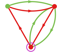
Imagine we have an opponent machine—like 3-state machine 1165—that usually forces a lose, i.e. limiting payoff –1 (for example about half the time when competing with other 3-state machines):
Now we can ask whether we can adaptively evolve a machine that will win against this opponent. In order to give our adaptive evolution process some “room to maneuver” we’ll use a 4-state machine. We can start with a random such machine, say
which “loses” (always having payoff –1) against machine 1165:
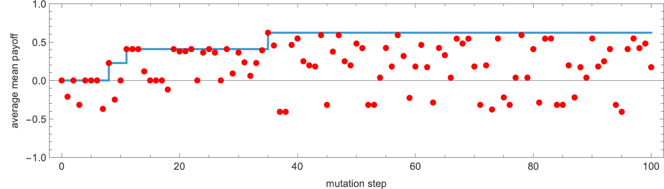
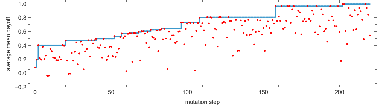
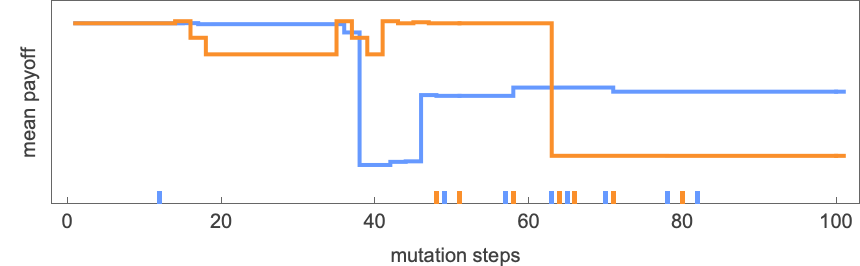
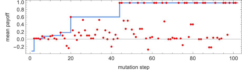
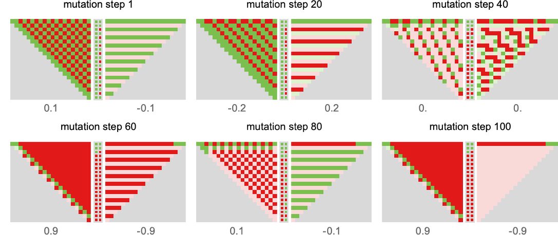
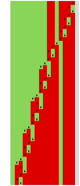
To do adaptive evolution, we now make successive random mutations to this machine, “accepting” a mutation if it doesn’t decrease the mean payoff, and otherwise rejecting it. The result is a typical “fitness curve” in which most mutations (indicated by red dots) don’t lead to improvement in the payoff—but there are some that lead to “breakthroughs” where the payoff increases (sometimes only by a small amount), with the payoff eventually reaching the maximum value of +1:
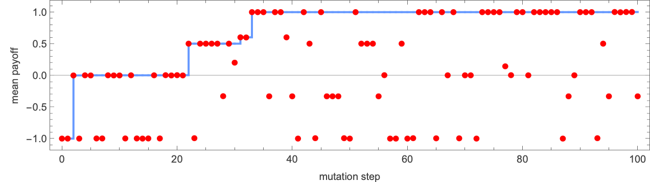
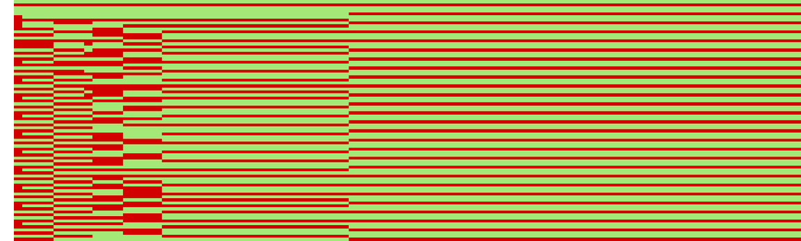
The various “breakthroughs” progressively converge on a “perfect solution” with payoff +1:
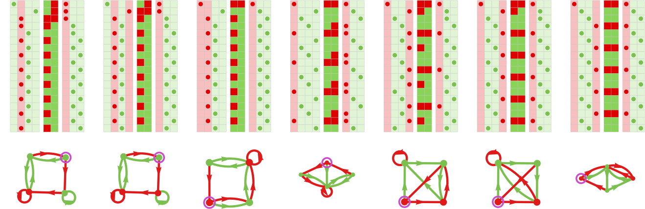
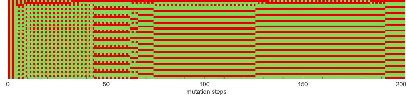
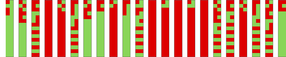
Concatenating the successive results over the course of the adaptive evolution process, we can see the eventual convergence to the perfect solution where the actions of the two agents always match:
With different random mutations, the “fitness curve” will be different in detail, though will have the same general form. And the same is true with different specific opponents.
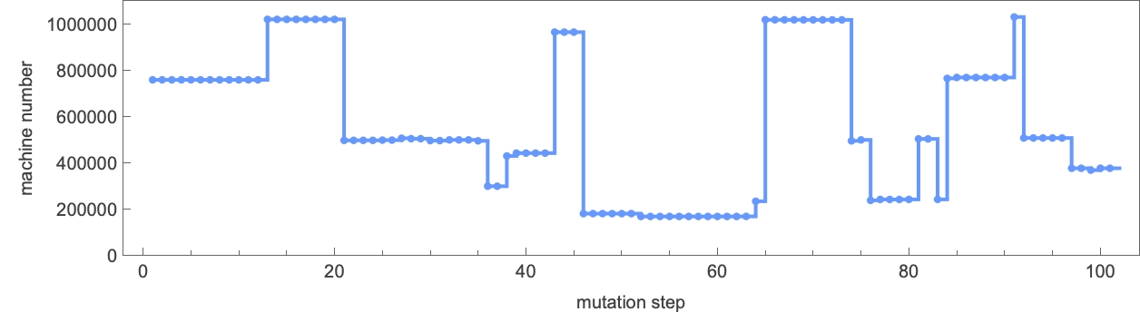
By the way, using our way of numbering finite state machines, we can make a plot of how the process of adaptive evolution “moves the machine around in rule space”:
But what happens if we do as we have done above, and ask about the mean payoff averaged over all possible finite-state-machine opponents of a given size? For example, how well can 4-state machines do against all possible 2-state machines?
Starting with the same random 4-state machine as before, a typical fitness curve is:
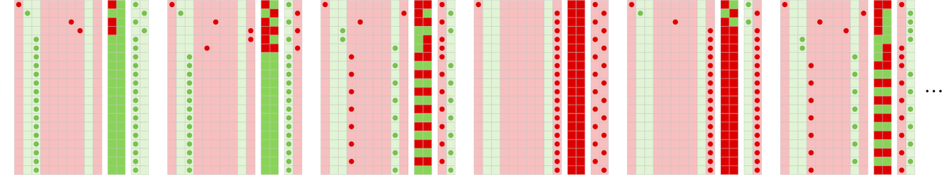
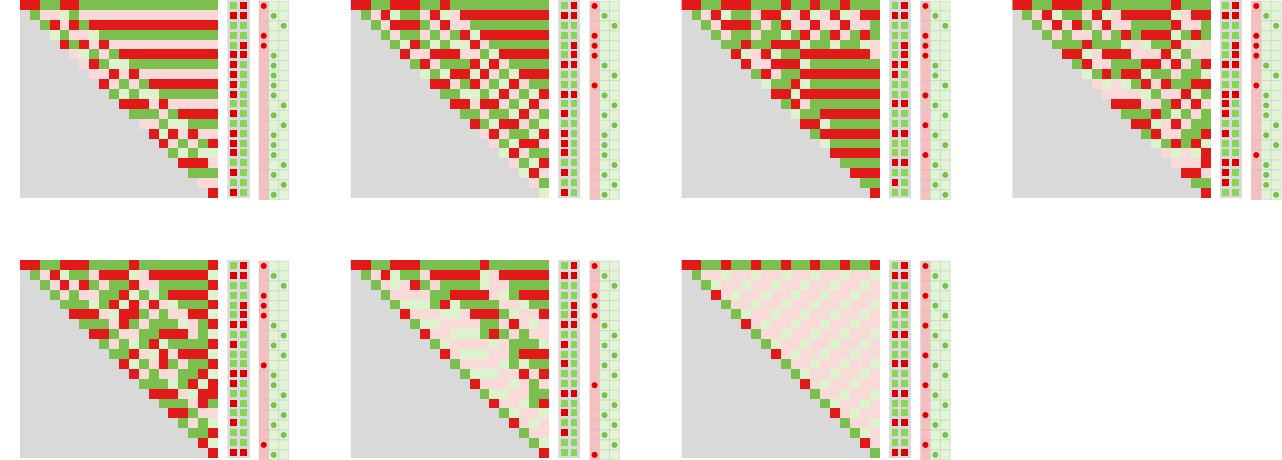
The fitness here increases, but never reaches +1. The behavior of successive “breakthrough” machines playing against all size-2 machines is:
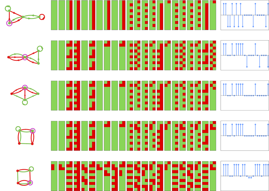
And we can see that even the best machine we get still loses to some of the 2-state machines, yielding in the end an average mean payoff of about 0.62.
So what happens if we look at machines that have more states? With 10 states, for example, it is possible to adaptively evolve to a machine that achieves limiting payoff +1 against every single 2-state machine:
The final machine obtained in this case
can be thought of as a kind of (2-state) “universal winner”—that ultimately wins against all 2-state machines:
How does it do it? In some sense the machine is big enough that it can have different “specialized parts” for different opponents. And if we look at how the machine behaves we indeed see that with different opponents the machine settles into different subsets of its complete space of states:
And even if we consider all 956 3-state machines as opponents, our machine continues to do well. It doesn’t win in all cases, but it still achieves an average mean payoff of +0.603:
Some examples where the machine doesn’t win—in effect because it doesn’t contain as a submachine something to deal with a particular opponent—include:
So far we’ve considered the adaptive evolution of a single machine competing either against a single fixed opponent, or against a collection of fixed opponents. But what if both the machine and its opponent are undergoing adaptive evolution?
For example, let’s say that on alternating adaptive evolution steps we do a mutation on a machine and on its opponent. We keep the mutation for each machine if the (mean) payoff for that machine does not decrease; otherwise we reject it.
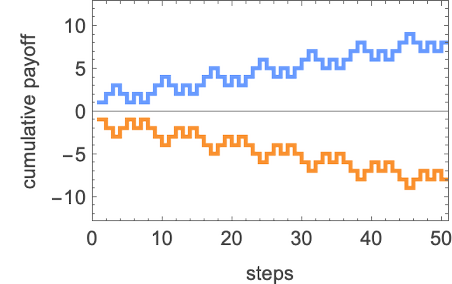
With this setup, here’s the evolution of mean payoffs for two (initially identical) 4-state machines:
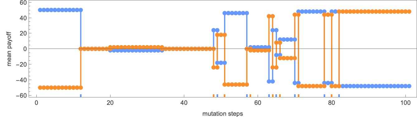
There are periods where one machine wins, and periods where its opponent wins—as visible in the actual successive behaviors of the machines:
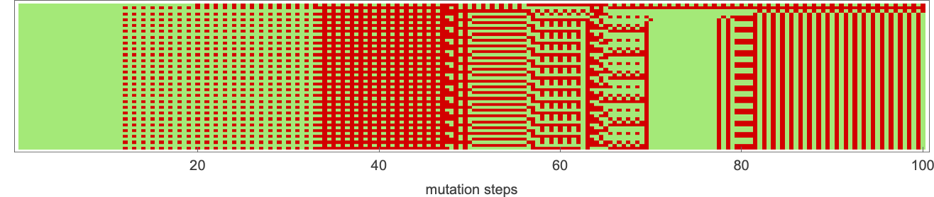
The actual machines found by adaptive evolution move around in rule space—soon losing memory of what they initially were:
Not much changes if the number of states in the machines change, or aren’t the same—though there is typically less alternation of winners for machines with more states, presumably because each individual mutation tends to have less effect on behavior if there are more states.
What About Prisoner’s Dilemma?
Everything we’ve done so far has been based on the particularly simple game of match-or-not (“matching pennies”). So what happens with other games? And in particular with the famous “prisoner’s dilemma” game? Here are the payoffs for this game
where in the usual narrative for the game one interprets ![]() as “defect” and
as “defect” and ![]() as “cooperate”.
as “cooperate”.
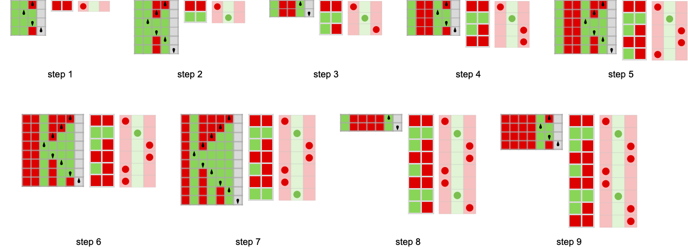
Just as above, we can imagine defining strategies for the prisoner’s dilemma game based on finite state machines. Here are a few examples of iterated games between 2-state machines—now with payoffs determined by the prisoner’s dilemma game:
In the case of match-or-not, it was visually easy to tell whether a particular payoff was ±1 or 0 just by seeing whether the actions of the agents matched at a particular step. Here it’s not quite so visually obvious.
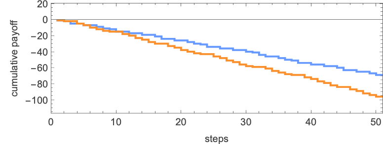
But using the payoffs for the prisoner’s dilemma game we can compute the cumulative payoffs for these examples (and, unlike in match-or-not, which is a zero-sum game, the payoffs for the two agents don’t sum to zero at each step):
Much as we did before, we can now consider competitions between agents whose strategies are based on all possible 2-state finite state machines (for match-or-not the zero-sum nature of the game makes the resulting array of payoffs symmetrical; here there’s symmetry only from the fact that the payoffs remain the same if one interchanges the roles of agent 1 and agent 2):
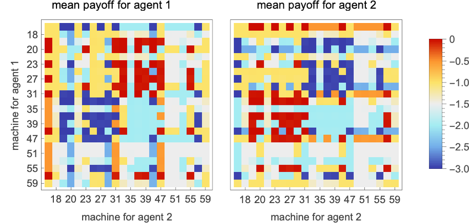
With this setup, we can now ask what machine is the “overall winner”—say in the sense that it has the largest average mean payoff playing against all other (distinct) 2-state machines:
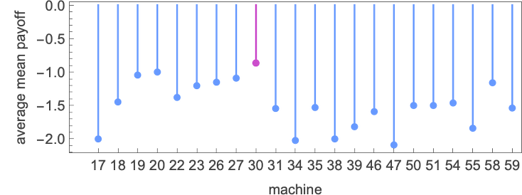
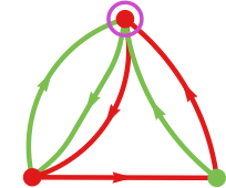
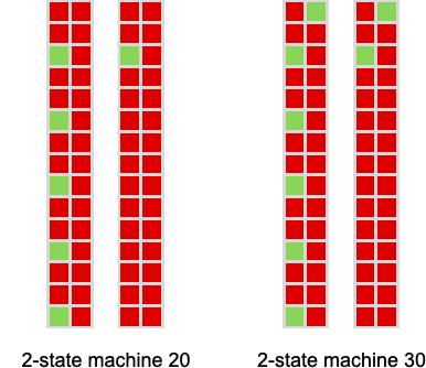
The answer turns out to be machine 30:
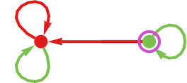
In the literature of prisoner’s dilemma this is often called “grim trigger”, because it yields a strategy that starts with ![]() , then repeats this until its opponent first gives
, then repeats this until its opponent first gives ![]() —after which it always gives
—after which it always gives ![]() .
.
Running this machine against all other 2-state machines we get the following behaviors
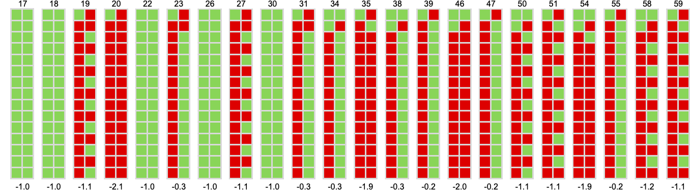
corresponding to the following mean payoffs:
Looking at the average mean payoff for all 2-state machines, the ranking of these machines is:
It’s notable that machine 22 (which corresponds to the famous “tit-for-tat” strategy)
is quite far down in this ranking, even though it’s often identified as the most successful in collections of human-suggested strategies.
The rankings we’ve just given are based on average mean payoffs obtained after many iterations of the prisoner’s dilemma game. But if we do only a few iterations, the rankings can be different:
Zooming in at the beginning we can then see that machine 30 only starts to win after 13 steps:
Machine 20 gives a constant average mean payoff of –1 obtained from
while machine 30 yields an average mean payoff given by –![]() –
– ![]() , limiting to –
, limiting to –![]() ≈ –0.86.
≈ –0.86.
So what about 3-state machines? This gives the average mean prisoner’s dilemma payoff for each of these machines:
The distribution of these average mean payoffs is:
The machines with the highest ultimate average mean payoffs are:
But this ordering emerges only after more than 500 steps
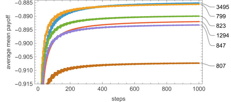
with the crossover of average mean payoffs being surprisingly complex:
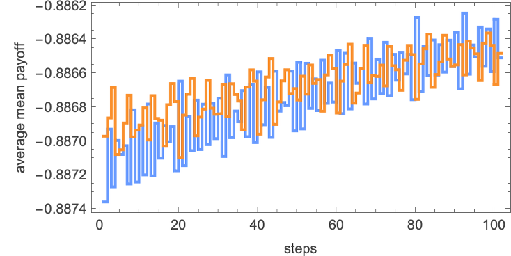
(The seemingly quite random variation of average mean payoffs reflects the combining of many different periods in the always-ultimately-periodic behavior of competitions between machines.)
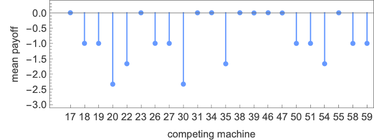
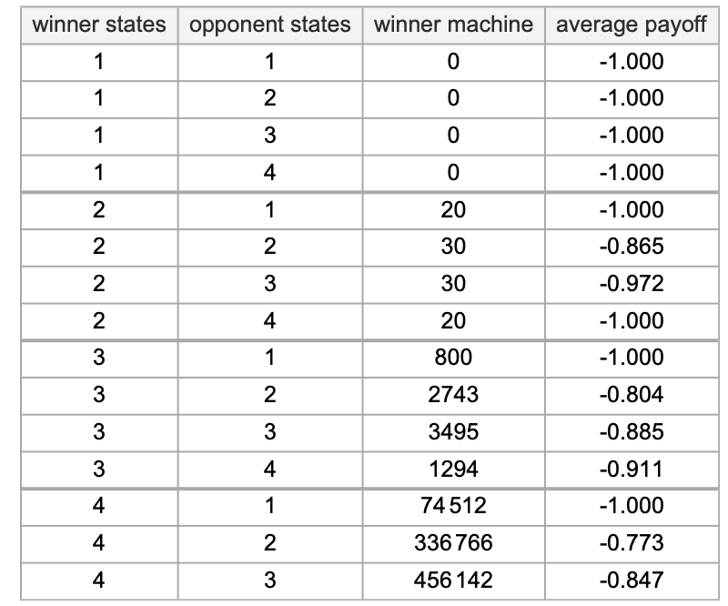
So how do 3-state machines do compared to 2-state machines in the prisoner’s dilemma game? Running 2-state machines against each other, machine 30 gets the highest average mean payoff of about –0.866. Meanwhile, for 3-state machines running against each other, the highest average mean payoff achieved is the very slightly smaller –0.885. What about 2-state machines running against 3-state ones? They don’t do well. Machine 30 does the best—but now it gives an average mean payoff not of –0.866 but instead of about –0.97.
But now, running 3-state machines against 2-state ones, the best average mean payoff is larger—about –0.80, as achieved by machine 2743
with the mean payoffs obtained by running it against each possible 2-state machines being:
How about 4-state machines? Running all these against 2-state machines, the overall winner is machine 336766 with average mean payoff –0.77:
The mean payoffs against each 2-state machine in this case

are very similar to those for the winning 3-state machine, the only different behaviors occurring when the opponents are 2-state machines 20 and 30:
Summarizing these results, the winning machines with small numbers of states that we’ve found for prisoner’s dilemma are:
But what about machines with more states—that we might find by adaptive evolution? Here’s an example of adaptive evolution for 10 states, competing against all 2-state machines:
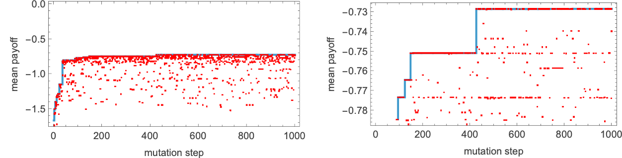
After 1000 steps of this adaptive evolution, we get the 10-state machine
with average mean payoff –0.73.
The behavior of this machine competing with all 2-state machines is:
The Space of All Possible Games
We’ve now looked at two specific examples of games—match-or-not and prisoner’s dilemma—and we’ve seen very similar phenomena in both cases. But what about other games?
If we allow payoffs –1 and +1 (as in match-or-not) there are a total of 256 possible games:
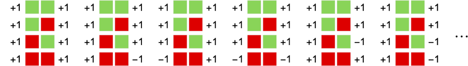
Of these, 16 are zero sum (like match-or-not)—in the sense that the sum of the payoffs for the two agents is always zero), and 16 are symmetric (like prisoner’s dilemma)—in the sense that the payoff for the two agents is always the same.
For each of the 256 possible games, we can compute the average mean payoffs for each possible 2-state finite state machine competing with all 2-state machines:
The winning average mean payoffs for these 256 games are always –1, 0 or +1:
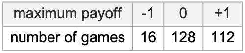
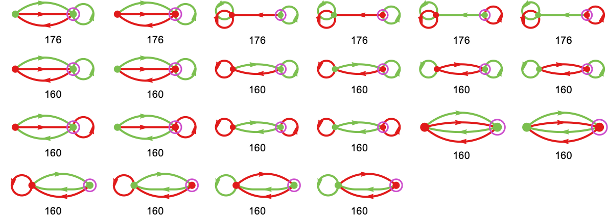
In most cases, many machines achieve the maximum payoff; across all games, this is the number of times each machine is a winner:
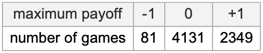
What about when we look at more games—for example ones with payoffs –1, 0, +1? There are 6561 such games. And the story is very much the same, with some slight differences:
Cellular Automaton Strategies
Everything we’ve done here so far has been based on using finite state machines as our source of strategies. Now we’re going to turn to another source of strategies: cellular automata.
The setup we’re going to use takes the actions of our agents to be determined by running cellular automaton rules. The basic idea is that at each step the initial conditions for the cellular automaton are given by the sequence of actions taken by the opponent so far. The next action of our agent is then determined by the value of the cell obtained by running the cellular automaton for as many steps as there were actions taken so far by the opponent.
More specifically, let’s say the rules for our cellular automaton are:
And let’s say the actions taken by the opponent so far have been:
Then the idea is to run the cellular automaton with these as initial conditions
and to extract the final cell value to determine the next action to take.
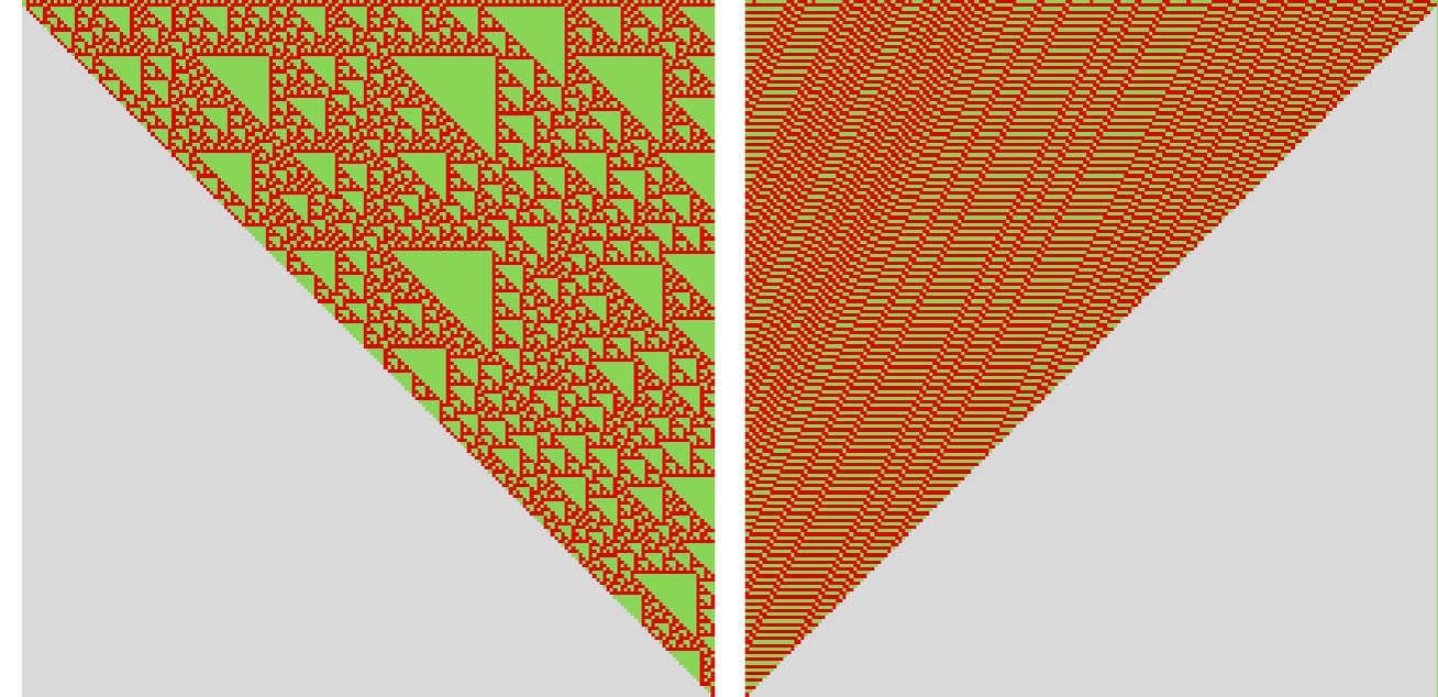
So, for example, if our two competing cellular automata have rules
then the successive steps in running them against each other give
where in our pictures everything about the second rule has been reversed. The actions taken on each step can now be read off either from the opponent initial conditions, or from the outer diagonals of the final pattern generated:
To analyze “competition” between rules we can assign payoffs, say from the match-or-not game:
And in this case we get the following cumulative payoffs:
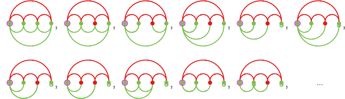
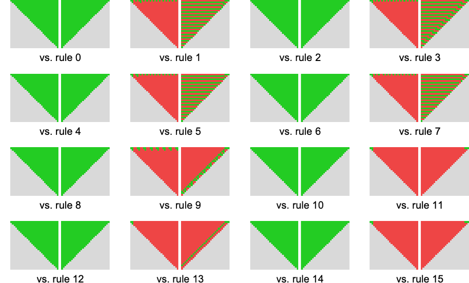
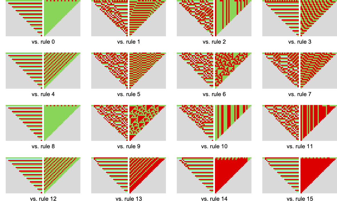
There are altogether 16 possible cellular automaton rules of the kind we’re using here:
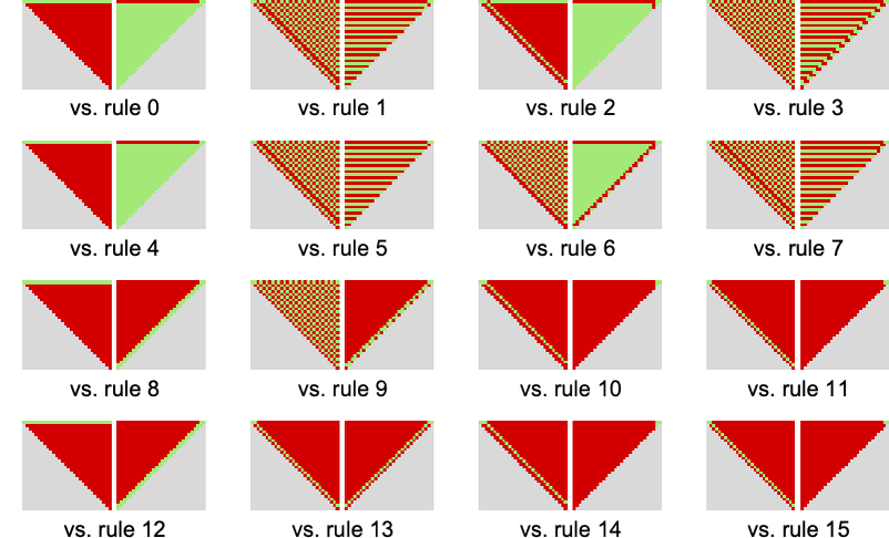
Running each one against every other we get the following array of limiting mean payoffs:
Some notable “competitions” include:
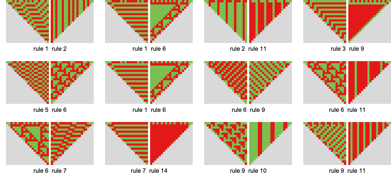
The cumulative mean (match-or-not) payoffs in these cases are:
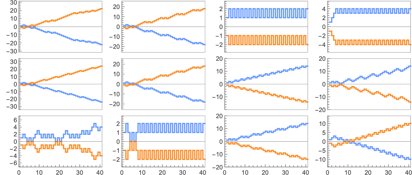
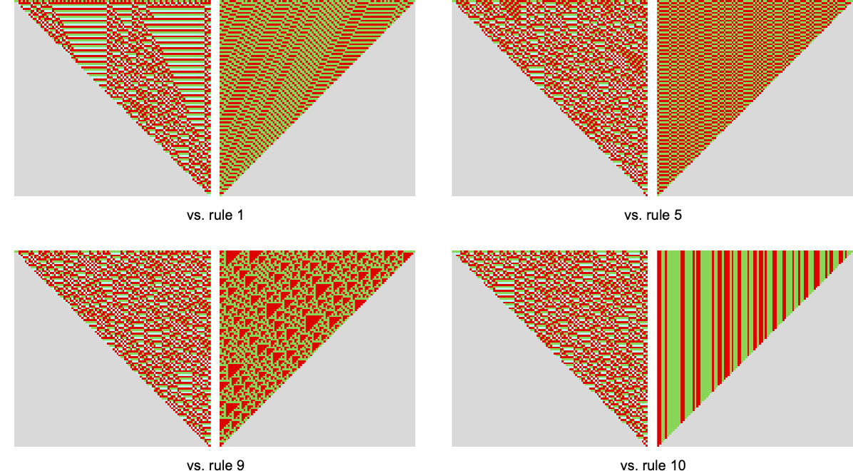
For most of these pairs of rules the winner quickly becomes clear. But for the case of rule 6 vs. rule 7 it’s more complicated—and after 500 steps it’s still not at all clear which rule will win:
The underlying behavior is:
On their own, these two rules behave in rather simple ways (indeed, rule 7 is just XOR):
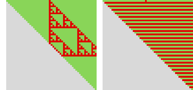
But when they’re set up in competition, the effective rule that emerges has much more complex—and apparently unpredictable—behavior, with no sign, for example, of periodicity.
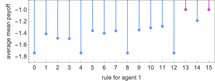
Looking across all the rules, the one with the largest average mean payoff turns out to be rule 14:
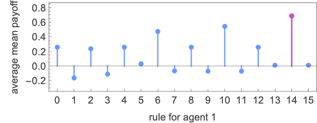
In a sense, rule 14 finds a very “simple solution”, generating either constant or period-2 behavior, and forcing its opponent to do likewise—and in the end giving an average mean payoff of exactly –![]() ≈ –0.69:
≈ –0.69:
What about with more complicated cellular automaton rules? Are the winners still ones with simple behavior?
Let’s look at the 3-color analogs of our cellular automaton rules. There are 332 = 19683 of these. And in each case we can “make a decision about the next action” by looking at the final value mod 2. Running all these rules against the 16 2-color rules the distribution of scores is:
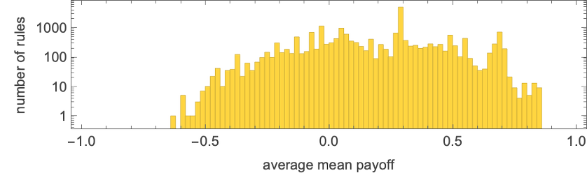
And once again the best-performing rules (such as rule 15911) behave in rather simple ways:
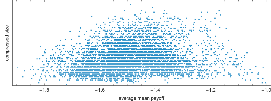
Looking—as we did for finite state machines—at the compressed size of patterns versus the average mean payoff in the corresponding competition
we see that the highest payoff rules tend to behave in simpler ways.
The rules with the most complicated behavior (at least by this measure) have average mean payoffs near zero. A typical example is rule 11948:
Some of the more complicated competitions in this case are:
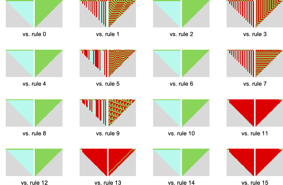
What about different games with different payoffs? The underlying behavior of particular rules competing with each other will always be the same. But their payoffs will be different. And so, for example, in prisoner’s dilemma, the cumulative payoffs for 2-color rule 6 vs. 2-color rule 7 are now:
Playing each 2-color rule against all others the average mean payoffs obtained are:
Rule 13 has the highest average mean payoff (of –1), and shows fairly simple behavior:
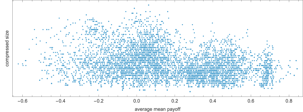
Looking at compressed size versus average mean payoff for games between 3-color and 2-color rules, the phenomenon of high payoff being associated with simpler behavior seems even more marked for prisoner’s dilemma than for match-or-not:
Cellular Automata vs. Finite State Machines
We’ve looked at finite state machines competing with finite state machines, and cellular automata competing with cellular automata. But what about cellular automata competing with finite state machines?
Here’s an example of a particular step in a competition between a cellular automaton and a finite state machine
and here are the cumulative payoffs in this case for the match-or-not game:
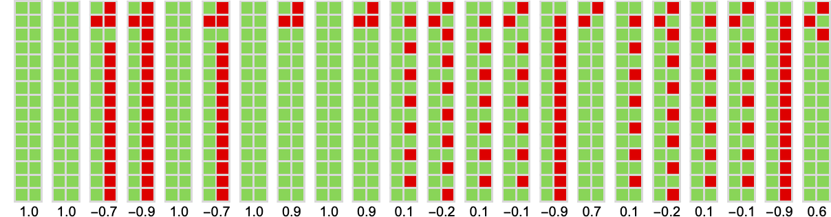
Running all 16 cellular automaton rules of this type against all 2-state finite state machines the mean payoffs are:

Averaging over all finite state machines, the mean payoffs for the possible cellular automata are:
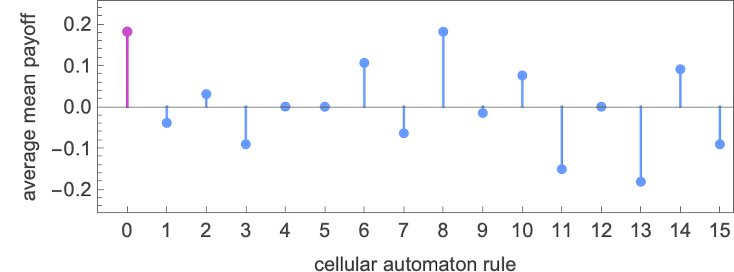
Rather boringly, the winning cellular automaton is rule 0, which generates ![]() in response to anything any finite state machine does:
in response to anything any finite state machine does:
This yields an average mean payoff of only +0.181. But what if we use 3-color cellular automata? Here are the average mean payoffs in that case—with the winning case highlighted:
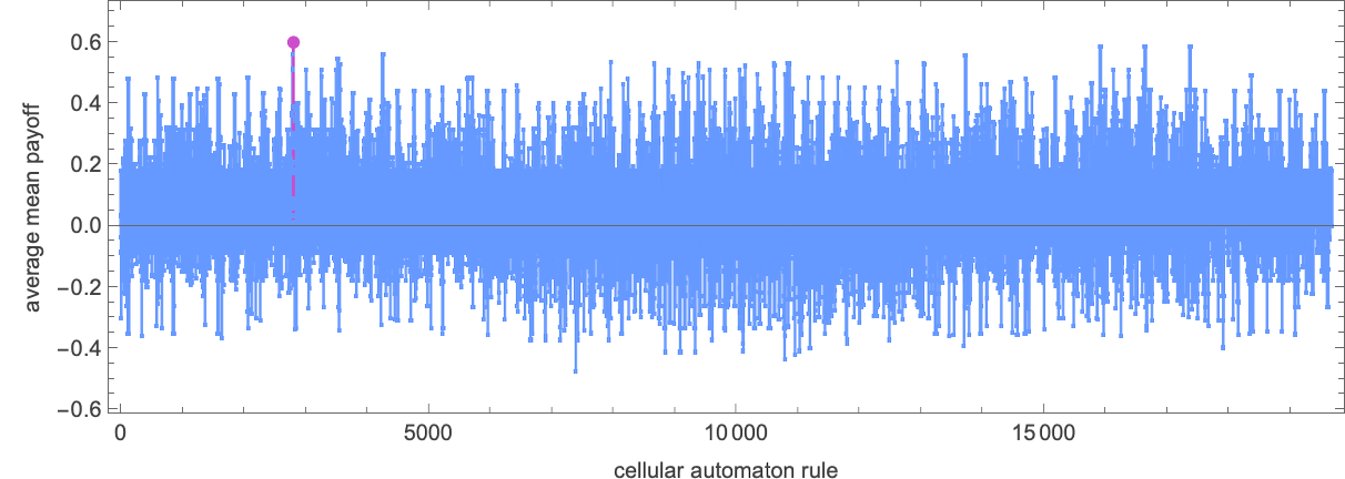
Summarizing the various competitions between different types of strategies, we see that—running against 2-state finite state machines—the most successful competitors are, by a small margin, 3-color cellular automata:
Adaptive Evolution of Cellular Automaton Strategies
Just as we did above for finite state machines, we can consider adaptive evolution of cellular automaton rules (which is also something I’ve studied in other contexts somewhat extensively elsewhere). As a first case, let’s consider adaptively evolving a 4-color cellular automaton rule to get the best mean payoff against the most successful 3-state finite state machine above, machine 1165. At each step of adaptive evolution, we’ll randomly change one of the
The “breakthroughs” correspond to the following rules:
And as is often the case, the early breakthroughs are somewhat complicated, but in the end the “solution” that emerges shows rather simple behavior—something we can see at least some evidence for if we put the results at successive mutation steps together:
What about adapting cellular automata to compete with other cellular automata? As an example, let’s use adaptive evolution to find a 6-color cellular automaton with the largest average mean payoff when competing with all 16 of the 2-color cellular automata we’ve considered. Here’s a typical fitness curve for this case:
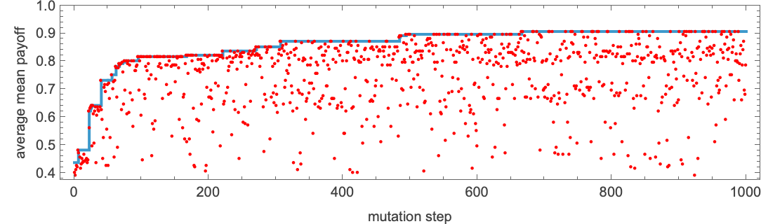
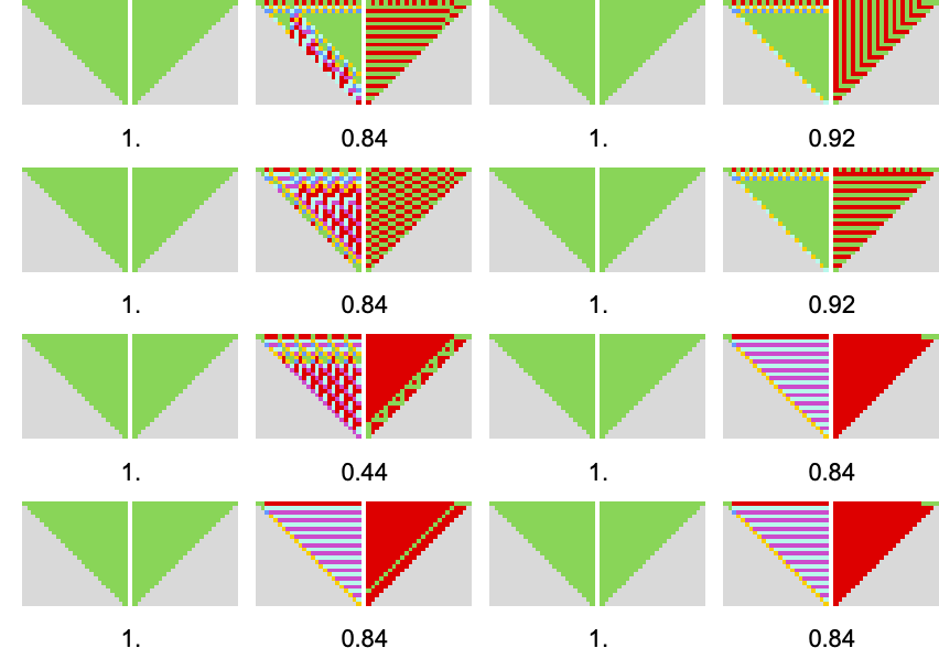
After 1000 mutation steps, it’s reached a rule that gives average mean payoff 0.91. And here’s what happens when that rule competes with all our 2-color rules:
What if (as for finite state machines above) both a rule and its opponent are undergoing adaptive evolution—say on alternating steps? Here’s an example of the successive payoffs one gets with a pair of 4-color rules:
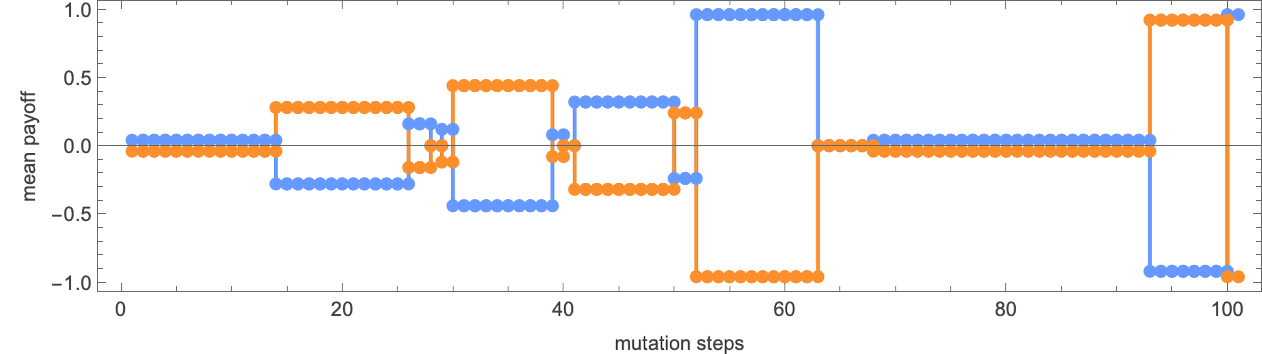
And here are the corresponding actual behaviors:
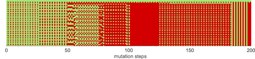
What are the underlying cellular automata doing? Here are results at a sequence of mutation steps—illustrating that adaptive evolution can select both rules with very simple behavior and ones with somewhat more complex behavior:
Turing Machine Strategies
We’ve looked at strategies based on finite state machines and strategies based on cellular automata. Now let’s talk about strategies based on Turing machines. For our purposes, we can think of Turing machines as in some ways interpolating between finite state machines and cellular automata—though they also introduce some entirely new features.
Our basic setup will be to use the opponent’s actions as initial values on a Turing machine tape, with the latest value on the right, which is where the Turing machine head is initially placed. We then run the Turing machine until its head goes further to the right than it’s ever gone before, at which point we determine the next action from the value that appears at the initial head position.
For example, consider a Turing machine defined by the rule:
Then imagine that the sequence of opponent actions so far is:
Running the Turing machine with this as its initial condition we get the following:
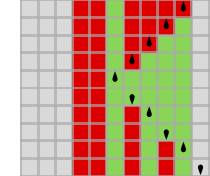
And from this we can then read off “the next move” according to our “Turing machine strategy”, in this case ![]() .
.
In our finite state machine and cellular automaton setups we did just one step of evolution for each step in our game. In our Turing machine setup, at every step in our game we’re running the Turing machine for as many steps as it takes for the head to go further to the right than it started.
Here’s what happens if we take a particular sample 3-state finite state machine
and have it compete with the Turing machine above:
With match-or-not the cumulative mean payoffs here are:
There are a total of 4096 Turing machines of the type we’re using here (with s = 2 states and k = 2 colors). Running each of these against our sample 3-state machine the mean payoffs in the match-or-not game for all the Turing machines are:
There are several Turing machines that have limiting mean payoffs of +1. An example is machine 2529:
There’s a tricky issue that comes up here, though. Our Turing machine strategy works by running a Turing machine until its head goes further to the right than it started—so that we can consider that it halts. But what if it never halts, as in:
For our purposes we’re just saying that in this case, the payoff is undefined. And if such an undefined payoff ever occurs in a particular game, we assume the mean payoff for the whole game is undefined—leaving a gap in the plot above.
What if we have Turing machines compete against, say, all distinct 2-state finite state machines? Here are the average mean payoffs in that case (the gaps are for machines that don’t halt):
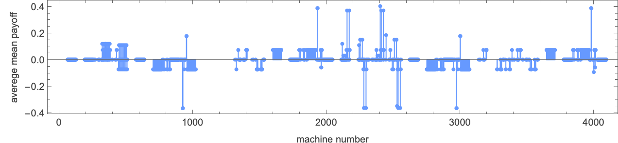
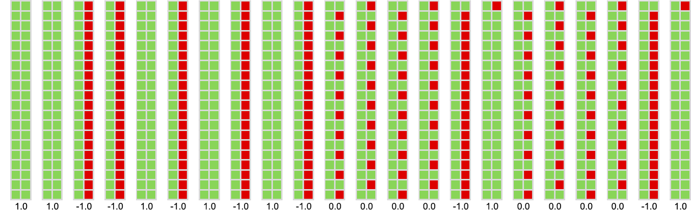
The maximum of +0.4 is achieved for Turing machine 2403
which yields the following behaviors and limiting payoffs when competing with each of the 22 distinct 2-state finite state machines:
So what about Turing machines competing with Turing machines? To keep things manageable, we can look at 1-state Turing machines, of which there are only 16 (with k = 2). Running each of these machines against each other, the array of mean payoffs is (the gray entries correspond to cases where one of the Turing machines doesn’t halt):
The average mean payoff for each of these machines is given by:
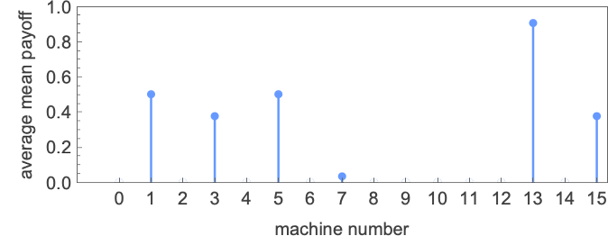
The “winner” among the machines is Turing machine 13:
Running this machine against all other s = 1, k = 2 Turing machines the behaviors we get are:
If we look at the cumulative payoffs, we see that many give mean payoffs that approach 1, though some do not, yielding in the end an average mean payoff of about +0.81:
A typical competition between 2-state Turing machines is
which yields a slightly more complicated pattern of cumulative payoffs:
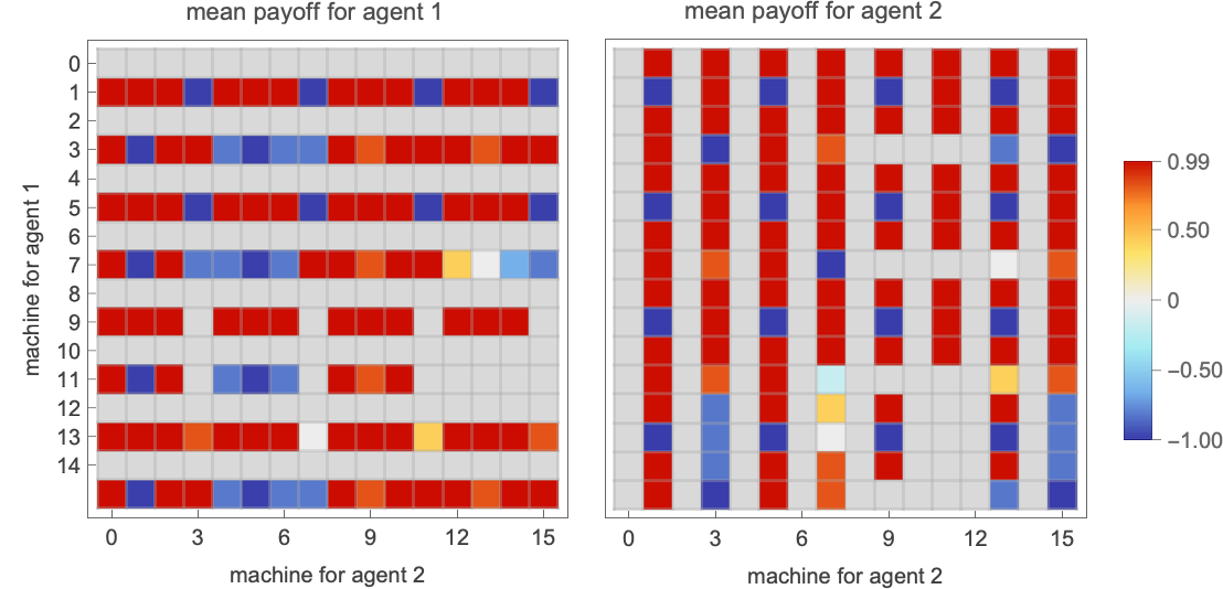
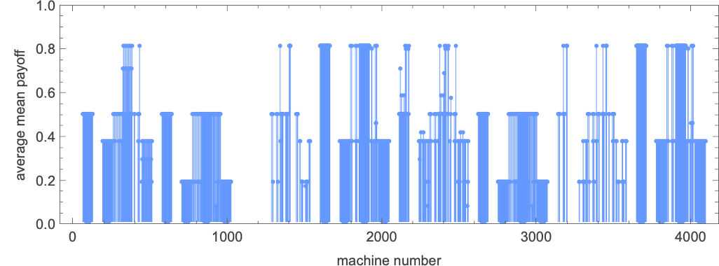
What happens if 2-state and 1-state Turing machines compete? Here’s the array of mean payoffs for all 4096 2-state machines running against the 16 1-state machines:

The average mean payoffs for 2-state machines are as follows—again with maximum 0.81:
Discussion
We’ve now seen many examples of the ruliology of competition. And, perhaps more than anything else, it’s now clear that if we look—ruliologically—at all possible programs of particular types, the picture of how competition works is quite complicated, even when all the programs involved are simple.
In a sense, this is a typical result of computational irreducibility: to know how competitions between programs will work out, there’s basically no choice but to run them and see what happens.
Sometimes the programs that win do so in very simple ways—in effect “exploiting simple hacks”. But in other cases, things are more complicated. Sometimes two competing programs with both show complex behavior, and in a sense, it’ll “just so happen” that one of them wins. But sometimes the win will be more systematic. And typically this happens because the behavior effectively plugs into some pocket of computational reducibility that systematically out-competes opponents of a certain type.
We’ve mostly looked at extremely simple programs which in some sense inevitably have to “expose the same rules” to every competitor. But particularly if we have a fairly small collection of competitors, a sufficiently large program can in effect expose a different part of its rules for different competitors, and so have a “customized substrategy” that separately wins against different possible competitors.
In looking at adaptive evolution of strategies we’ve often dealt with larger programs. And we’ve typically seen that the adaptive evolution can be quite successful at finding winning strategies. But—as is typically the case with adaptive evolution—there’s no obvious way to “describe the mechanism” of the strategies that are produced. Instead, it’s more like what we’ve seen in other studies of adaptive evolution: the process of evolution puts together certain “lumps of irreducible computation” that in our case here in effect “just happen” to be competitively successful.
Different games—corresponding to different patterns of payoffs—lead to results that are different in detail. And if one constructs a detailed narrative about the course of a game, it may well seem different for different games. But at an overall level, there seems to be remarkable similarity between different games—and the key phenomena seem very much the same.
What does this all say about practical situations where there’s competition between agents? One thing is that it’s typically going to be difficult to “predict in advance” or “prove a theorem” about what the best strategy will be. There’s enough computational irreducibility that one will basically just have to try running different competitions and seeing what happens. And in a sense the very diversity of behavior we’ve seen here supports the idea that ruliological investigation is critical. Finding some simple parametrization of possible strategies won’t be enough to get an accurate sense of everything that can happen. There’s no choice but to systematically enumerate some version of “all computationally possible strategies”. Which is what we can do in our ruliological investigations.
And, yes, what we’ve done here just scratches the surface of studying the ruliology of competition. For a start, one can scale up the size of the programs, and see what new phenomena occur. One can expect that mostly things will be the same—with computational irreducibility the dominant force. But there may be new and unexpected pockets of reducibility, perhaps each with their own “paths to competitive success”.
One can also imagine investigating different kinds of computational systems—that serve as metamodels appropriate for different applications. The Principle of Computational Equivalence suggests that there’ll be a certain universality to the overall results. But details will be different. And those details will potentially be important, particularly in interpreting results for very different domains. Even if what matters for ultimate purposes of competition is well captured by finite state machines—or a cellular automata—the way one gets to these from microscopic biology, human decision making, societal interactions, AI competition, etc. may be very different.
Historical & Personal Notes
There’s a long history to formal studies of games—and indeed early developments in areas like combinatorics and probability were largely driven by them. The modern field known as game theory emerged in the 1940s, concentrating on the question of optimal strategies given particular patterns of payoffs. Most often the idea is to analyze what happens when each player makes a single move—albeit perhaps a probabilistic one, with averages taken over many instances. Fairly complete (though sometimes complicated) mathematical results have been derived for this kind of setup (and are now, for example, implemented in the Wolfram Language). But what about repeated, or iterated, games of the kind we’ve been discussing here? In the early days of game theory there was discussion about defining strategies as arbitrary mappings from histories to actions—and various rather abstract mathematical results were proved, particularly for applications in economics.
But by the 1970s there started to emerge the idea that one should model agents as having “bounded rationality”, and corresponding to limited computational systems. And by the end of the 1970s computer experiments were being done on competition between what amounted to simple programs. A notable example was the tournament organized by Bob Axelrod for the prisoner’s dilemma game. In this tournament, a collection of particular programs were submitted by different individuals, and run against each other. The conclusion was that the “tit-for-tat” strategy (that can be thought of as a finite state machine) came out best—a result from which much has been made about the value of cooperation, etc.
I must admit that I was always suspicious of the result. It seemed very unscientific to have just looked at programs people happened to have submitted for the tournament. Why not instead systematically enumerate all possible programs and see what happens? In my own work—starting at the beginning of the 1980s—I was routinely doing this kind of thing, particularly for cellular automata. I always found the setup for game theory a little arbitrary, and fiddly, and I was discovering more than I could keep up with just investigating the behavior of individual programs, without trying to have them compete with each other. Still, finally, in the mid-1990s, I did have a look at what happens when a range of possible programs (in that case, cellular automata) compete with each other. I summarized the result in a small note at the end of my book A New Kind of Science:

I always meant to come back and look at this in more detail. And finally my recent work in the foundations of biological evolution made me think it was time to do it. I found out that there was some literature on using models like finite state machines as strategies for iterated games. But so far as I could tell, the kind of systematic ruliological investigation I had imagined had never been done. Which is why I recently decided it was finally time to do it…
Thanks
Thanks to Willem Nielsen, Brian Ashiundu and Júlia Campolim of the Wolfram Institute for their extensive help. Several participants at our summer programs have done projects about games between programs that I’ve suggested: Rodrigo Bazaes, Kantaporn Danchaivijitr and Aziz Sahibnazarov. Over the course of many years, I’ve discussed game theory and related ideas with quite a few people, including Brian Arthur, Bob Axelrod, Seth Chandler, Roger Germundsson, Paul Harrald, Jozsef Konczer, Pedro Marquez-Zacarias, Eric Maskin, Zsombor Méder, Chrystopher Nehaniv, Scott Page, Jordan Pollack, John Maynard Smith, Stan Reiter, Nassim Taleb, Valeriu Ungureanu and Marc Vicuna. (Notable game theorist John Nash was a long-time user of what’s now Wolfram Language, and attended conferences about it, but I never personally met him.)
Posted in: Artificial Intelligence, Computational Science, Life Science, Ruliology