The Leading Edge of 2023 Technology … and Beyond
Today we’re launching Version 13.3 of Wolfram Language and Mathematica—both available immediately on desktop and cloud. It’s only been 196 days since we released Version 13.2, but there’s a lot that’s new, not least a whole subsystem around LLMs.
Last Friday (June 23) we celebrated 35 years since Version 1.0 of Mathematica (and what’s now Wolfram Language). And to me it’s incredible how far we’ve come in these 35 years—yet how consistent we’ve been in our mission and goals, and how well we’ve been able to just keep building on the foundations we created all those years ago.
And when it comes to what’s now Wolfram Language, there’s a wonderful timelessness to it. We’ve worked very hard to make its design as clean and coherent as possible—and to make it a timeless way to elegantly represent computation and everything that can be described through it.
Last Friday I fired up Version 1 on an old Mac SE/30 computer (with 2.5 megabytes of memory), and it was a thrill see functions like Plot and NestList work just as they would today—albeit a lot slower. And it was wonderful to be able to take (on a floppy disk) the notebook I created with Version 1 and have it immediately come to life on a modern computer.
But even as we’ve maintained compatibility over all these years, the scope of our system has grown out of all recognition—with everything in Version 1 now occupying but a small sliver of the whole range of functionality of the modern Wolfram Language:

So much about Mathematica was ahead of its time in 1988, and perhaps even more about Mathematica and the Wolfram Language is ahead of its time today, 35 years later. From the whole idea of symbolic programming, to the concept of notebooks, the universal applicability of symbolic expressions, the notion of computational knowledge, and concepts like instant APIs and so much more, we’ve been energetically continuing to push the frontier over all these years.
Our long-term objective has been to build a full-scale computational language that can represent everything computationally, in a way that’s effective for both computers and humans. And now—in 2023—there’s a new significance to this. Because with the advent of LLMs our language has become a unique bridge between humans, AIs and computation.
The attributes that make Wolfram Language easy for humans to write, yet rich in expressive power, also make it ideal for LLMs to write. And—unlike traditional programming languages— Wolfram Language is intended not only for humans to write, but also to read and think in. So it becomes the medium through which humans can confirm or correct what LLMs do, to deliver computational language code that can be confidently assembled into a larger system.
The Wolfram Language wasn’t originally designed with the recent success of LLMs in mind. But I think it’s a tribute to the strength of its design that it now fits so well with LLMs—with so much synergy. The Wolfram Language is important to LLMs—in providing a way to access computation and computational knowledge from within the LLM. But LLMs are also important to Wolfram Language—in providing a rich linguistic interface to the language.
We’ve always built—and deployed—Wolfram Language so it can be accessible to as many people as possible. But the advent of LLMs—and our new Chat Notebooks—opens up Wolfram Language to vastly more people. Wolfram|Alpha lets anyone use natural language—without prior knowledge—to get questions answered. Now with LLMs it’s possible to use natural language to start defining potential elaborate computations.
As soon as you’ve formulated your thoughts in computational terms, you can immediately “explain them to an LLM”, and have it produce precise Wolfram Language code. Often when you look at that code you’ll realize you didn’t explain yourself quite right, and either the LLM or you can tighten up your code. But anyone—without any prior knowledge—can now get started producing serious Wolfram Language code. And that’s very important in seeing Wolfram Language realize its potential to drive “computational X” for the widest possible range of
But while LLMs are “the biggest single story” in Version 13.3, there’s a lot else in Version 13.3 too—delivering the latest from our long-term research and development pipeline. So, yes, in Version 13.3 there’s new functionality not only in LLMs but also in many “classic” areas—as well as in new areas having nothing to do with LLMs.
Across the 35 years since Version 1 we’ve been able to continue accelerating our research and development process, year by year building on the functionality and automation we’ve created. And we’ve also continually honed our actual process of research and development—for the past 5 years sharing our design meetings on open livestreams.
Version 13.3 is—from its name—an “incremental release”. But—particularly with its new LLM functionality—it continues our tradition of delivering a long list of important advances and updates, even in incremental releases.
LLM Tech Comes to Wolfram Language
LLMs make possible many important new things in the Wolfram Language. And since I’ve been discussing these in a series of recent posts, I’ll just give only a fairly short summary here. More details are in the other posts, both ones that have appeared, and ones that will appear soon.
To ensure you have the latest Chat Notebook functionality installed and available, use:
The most immediately visible LLM tech in Version 13.3 is Chat Notebooks. Go to

You might not like some details of what got done (do you really want those boldface labels?) but I consider this pretty impressive. And it’s a great example of using an LLM as a “linguistic interface” with common sense, that can generate precise computational language, which can then be run to get a result.
This is all very new technology, so we don’t yet know what patterns of usage will work best. But I think it’s going to go like this. First, you have to think computationally about whatever you’re trying to do. Then you tell it to the LLM, and it’ll produce Wolfram Language code that represents what it thinks you want to do. You might just run that code (or the Chat Notebook will do it for you), and see if it produces what you want. Or you might read the code, and see if it’s what you want. But either way, you’ll be using computational language—Wolfram Language—as the medium to formalize and express what you’re trying to do.
When you’re doing something you’re familiar with, it’ll almost always be faster and better to think directly in Wolfram Language, and just enter the computational language code you want. But if you’re exploring something new, or just getting started on something, the LLM is likely to be a really valuable way to “get you to first code”, and to start the process of crispening up what you want in computational terms.
If the LLM doesn’t do exactly what you want, then you can tell it what it did wrong, and it’ll try to correct it—though sometimes you can end up doing a lot of explaining and having quite a long dialog (and, yes, it’s often vastly easier just to type Wolfram Language code yourself):


Sometimes the LLM will notice for itself that something went wrong, and try changing its code, and rerunning it:

And even if it didn’t write a piece of code itself, it’s pretty good at piping up to explain what’s going on when an error is generated:

And actually it’s got a big advantage here, because “under the hood” it can look at lots of details (like stack trace, error documentation, etc.) that humans usually don’t bother with.
To support all this interaction with LLMs, there’s all kinds of new structure in the Wolfram Language. In Chat Notebooks there are chat cells, and there are chatblocks (indicated by gray bars, and generating with ~) that delimit the range of chat cells that will be fed to the LLM when you press shiftenter on a new chat cell. And, by the way, the whole mechanism of cells, cell groups, etc. that we invented 36 years ago now turns out to be extremely powerful as a foundation for Chat Notebooks.
One can think of the LLM as a kind of “alternate evaluator” in the notebook. And there are various ways to set up and control it. The most immediate is in the menu associated with every chat cell and every chatblock (and also available in the notebook toolbar):

The first items here let you define the “persona” for the LLM. Is it going to act as a Code Assistant that writes code and comments on it? Or is it just going to be a Code Writer, that writes code without being wordy about it? Then there are some “fun” personas—like Wolfie and Birdnardo—that respond “with an attitude”. The Advanced Settings let you do things like set the underlying LLM model you want to use—and also what tools (like Wolfram Language code evaluation) you want to connect to it.
Ultimately personas are mostly just special prompts for the LLM (together, sometimes with tools, etc.) And one of the new things we’ve recently launched to support LLMs is the Wolfram Prompt Repository:

The Prompt Repository contains several kinds of prompts. The first are personas, which are used to “style” and otherwise inform chat interactions. But then there are two other types of prompts: function prompts, and modifier prompts.
Function prompts are for getting the LLM to do something specific, like summarize a piece of text, or suggest a joke (it’s not terribly good at that). Modifier prompts are for determining how the LLM should modify its output, for example translating into a different human language, or keeping it to a certain length.
You can pull in function prompts from the repository into a Chat Notebook by using !, and modifier prompts using #. There’s also a ^ notation for saying that you want the “input” to the function prompt to be the cell above:

This is how you can access LLM functionality from within a Chat Notebook. But there’s also a whole symbolic programmatic way to access LLMs that we’ve added to the Wolfram Language. Central to this is LLMFunction, which acts very much like a Wolfram Language pure function, except that it gets “evaluated” not by the Wolfram Language kernel, but by an LLM:
You can access a function prompt from the Prompt Repository using LLMResourceFunction:

There’s also a symbolic representation for chats. Here’s an empty chat:

And here now we “say something”, and the LLM responds:

There’s lots of depth to both Chat Notebooks and LLM functions—as I’ve described elsewhere. There’s LLMExampleFunction for getting an LLM to follow examples you give. There’s LLMTool for giving an LLM a way to call functions in the Wolfram Language as “tools”. And there’s LLMSynthesize which provides raw access to the LLM as its text completion and other capabilities. (And controlling all of this is $LLMEvaluator which defines the default LLM configuration to use, as specified by an LLMConfiguration object.)
I consider it rather impressive that we’ve been able to get to the level of support for LLMs that we have in Version 13.3 in less than six months (along with building things like the Wolfram Plugin for ChatGPT, and the Wolfram ChatGPT Plugin Kit). But there’s going to be more to come, with LLM functionality increasingly integrated into Wolfram Language and Notebooks, and, yes, Wolfram Language functionality increasingly integrated as a tool into LLMs.
Line, Surface and Contour Integration
“Find the integral of the function ___” is a typical core thing one wants to do in calculus. And in Mathematica and the Wolfram Language that’s achieved with Integrate. But particularly in applications of calculus, it’s common to want to ask slightly more elaborate questions, like “What’s the integral of ___ over the region ___?”, or “What’s the integral of ___ along the line ___?”
Almost a decade ago (in Version 10) we introduced a way to specify integration over regions—just by giving the region “geometrically” as the domain of the integral:

It had always been possible to write out such an integral in “standard Integrate” form

but the region specification is much more convenient—as well as being much more efficient to process.
Finding an integral along a line is also something that can ultimately be done in “standard Integrate” form. And if you have an explicit (parametric) formula for the line this is typically fairly straightforward. But if the line is specified in a geometrical way then there’s real work to do to even set up the problem in “standard Integrate” form. So in Version 13.3 we’re introducing the function LineIntegrate to automate this.
LineIntegrate can deal with integrating both scalar and vector functions over lines. Here’s an example where the line is just a straight line:

But LineIntegrate also works for lines that aren’t straight, like this parametrically specified one:

To compute the integral also requires finding the tangent vector at every point on the curve—but LineIntegrate automatically does that:

Line integrals are common in applications of calculus to physics. But perhaps even more common are surface integrals, representing for example total flux through a surface. And in Version 13.3 we’re introducing SurfaceIntegrate. Here’s a fairly straightforward integral of flux that goes radially outward through a sphere:
Here’s a more complicated case:


And here’s what the actual vector field looks like on the surface of the dodecahedron:

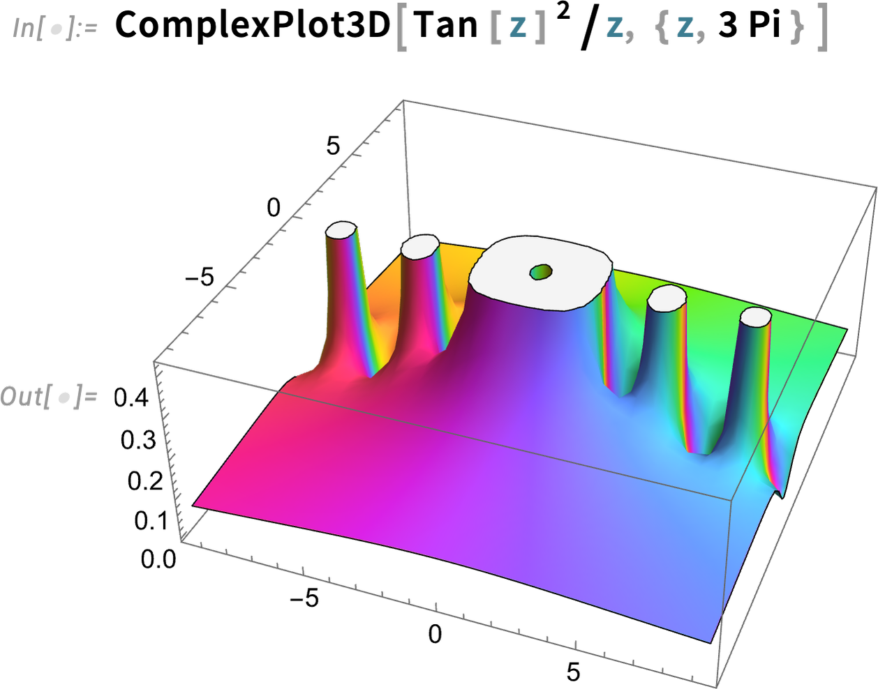
LineIntegrate and SurfaceIntegrate deal with integrating scalar and vector functions in Euclidean space. But in Version 13.3 we’re also handling another kind of integration: contour integration in the complex plane.
We can start with a classic contour integral—illustrating Cauchy’s theorem:
Here’s a slightly more elaborate complex function
and here’s its integral around a circular contour:

Needless to say, this still gives the same result, since the new contour still encloses the same poles:

More impressively, here’s the result for an arbitrary radius of contour:

And here’s a plot of the (imaginary part of the) result:

Contours can be of any shape:

The result for the contour integral depends on whether the pole is inside the “Pac-Man”:

Another Milestone for Special Functions
One can think of special functions as a way of “modularizing” mathematical results. It’s often a challenge to know that something can be expressed in terms of special functions. But once one’s done this, one can immediately apply the independent knowledge that exists about the special functions.
Even in Version 1.0 we already supported many special functions. And over the years we’ve added support for many more—to the point where we now cover everything that might reasonably be considered a “classical” special function. But in recent years we’ve also been tackling more general special functions. They’re mathematically more complex, but each one we successfully cover makes a new collection of problems accessible to exact solution and reliable numerical and symbolic computation.
Most of the “classic” special functions—like Bessel functions, Legendre functions, elliptic integrals, etc.—are in the end univariate hypergeometric functions. But one important frontier in “general special functions” are those corresponding to bivariate hypergeometric functions. And already in Version 4.0 (1999) we introduced one example of such as a function: AppellF1. And, yes, it’s taken a while, but now in Version 13.3 we’ve finally finished doing the math and creating the algorithms to introduce AppellF2, AppellF3 and AppellF4.
On the face of it, it’s just another function—with lots of arguments—whose value we can find to any precision:
Occasionally it has a closed form:

But despite its mathematical sophistication, plots of it tend to look fairly uninspiring:

Series expansions begin to show a little more:

And ultimately this is a function that solves a pair of PDEs that can be seen as a generalization to two variables of the univariate hypergeometric ODE. So what other generalizations are possible? Paul Appell spent many years around the turn of the twentieth century looking—and came up with just four, which as of Version 13.3 now all appear in the Wolfram Language, as AppellF1, AppellF2, AppellF3 and AppellF4.
To make special functions useful in the Wolfram Language they need to be “knitted” into other capabilities of the language—from numerical evaluation to series expansion, calculus, equation solving, and integral transforms. And in Version 13.3 we’ve passed another special function milestone, around integral transforms.
When I started using special functions in the 1970s the main source of information about them tended to be a small number of handbooks that had been assembled through decades of work. When we began to build Mathematica and what’s now the Wolfram Language, one of our goals was to subsume the information in such handbooks. And over the years that’s exactly what we’ve achieved—for integrals, sums, differential equations, etc. But one of the holdouts has been integral transforms for special functions. And, yes, we’ve covered a great many of these. But there are exotic examples that can often only “coincidentally” be done in closed form—and that in the past have only been found in books of tables.
But now in Version 13.3 we can do cases like:

And in fact we believe that in Version 13.3 we’ve reached the edge of what’s ever been figured out about Laplace transforms for special functions. The most extensive handbook—finally published in 1973—runs to about 400 pages. A few years ago we could do about 55% of the forward Laplace transforms in the book, and 31% of the inverse ones. But now in Version 13.3 we can do 100% of the ones that we can verify as correct (and, yes, there are definitely some mistakes in the book). It’s the end of a long journey, and a satisfying achievement in the quest to make as much mathematical knowledge as possible automatically computable.
Finite Fields!
Ever since Version 1.0 we’ve been able to do things like factoring polynomials modulo primes. And many packages have been developed that handle specific aspects of finite fields. But in Version 13.3 we now have complete, consistent coverage of all finite fields—and operations with them.
Here’s our symbolic representation of the field of integers modulo 5 (AKA ℤ5 or GF(5)):

And here are symbolic representations of the elements of this field—which in this particular case can be rather trivially identified with ordinary integers mod 5:

Arithmetic immediately works on these symbolic elements:

But where things get a bit trickier is when we’re dealing with prime-power fields. We represent the field GF(23) symbolically as:

But now the elements of this field no longer have a direct correspondence with ordinary integers. We can still assign “indices” to them, though (with elements 0 and 1 being the additive and multiplicative identities). So here’s an example of an operation in this field:

But what actually is this result? Well, it’s an element of the finite field—with index 4—represented internally in the form:

The little box opens out to show the symbolic FiniteField construct:

And we can extract properties of the element, like its index:

So here, for example, are the complete addition and multiplication tables for this field:

For the field GF(72) these look a little more complicated:

There are various number-theoretic-like functions that one can compute for elements of finite fields. Here’s an element of GF(510):

The multiplicative order of this (i.e. power of it that gives 1) is quite large:

Here’s its minimal polynomial:

But where finite fields really begin to come into their own is when one looks at polynomials over them. Here, for example, is factoring over GF(32):
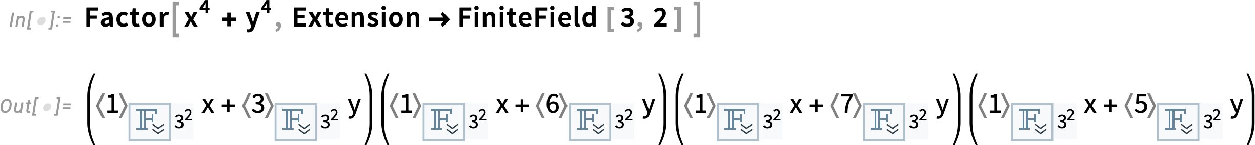
Expanding this gives a finite-field-style representation of the original polynomial:

Here’s the result of expanding a power of a polynomial over GF(32):

More, Stronger Computational Geometry
We originally introduced computational geometry in a serious way into the Wolfram Language a decade ago. And ever since then we’ve been building more and more capabilities in computational geometry.
We’ve had RegionDistance for computing the distance from a point to a region for a decade. In Version 13.3 we’ve now extended RegionDistance so it can also compute the shortest distance between two regions:
We’ve also introduced RegionFarthestDistance which computes the furthest distance between any two points in two given regions:
Another new function in Version 13.3 is RegionHausdorffDistance which computes the largest of all shortest distances between points in two regions; in this case it gives a closed form:

Another pair of new functions in Version 13.3 are InscribedBall and CircumscribedBall—which give (n-dimensional) spheres that, respectively, just fit inside and outside regions you give:

In the past several versions, we’ve added functionality that combines geo computation with computational geometry. Version 13.3 has the beginning of another initiative—introducing abstract spherical geometry:
This works for spheres in any number of dimensions:

In addition to adding functionality, Version 13.3 also brings significant speed enhancements (often 10x or more) to some core operations in 2D computational geometry—making things like computing this fast even though it involves complicated regions:

Visualizations Begin to Come Alive
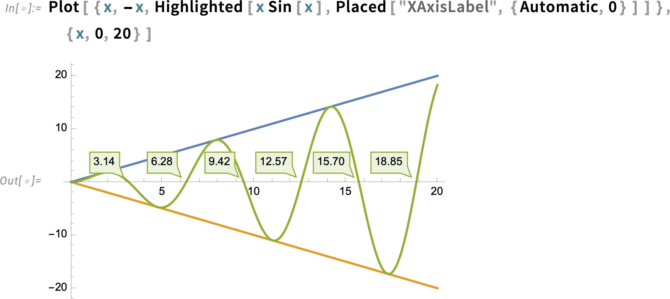
A great long-term strength of the Wolfram Language has been its ability to produce insightful visualizations in a highly automated way. In Version 13.3 we’re taking this further, by adding automatic “live highlighting”. Here’s a simple example, just using the function Plot. Instead of just producing static curves, Plot now automatically generates a visualization with interactive highlighting:
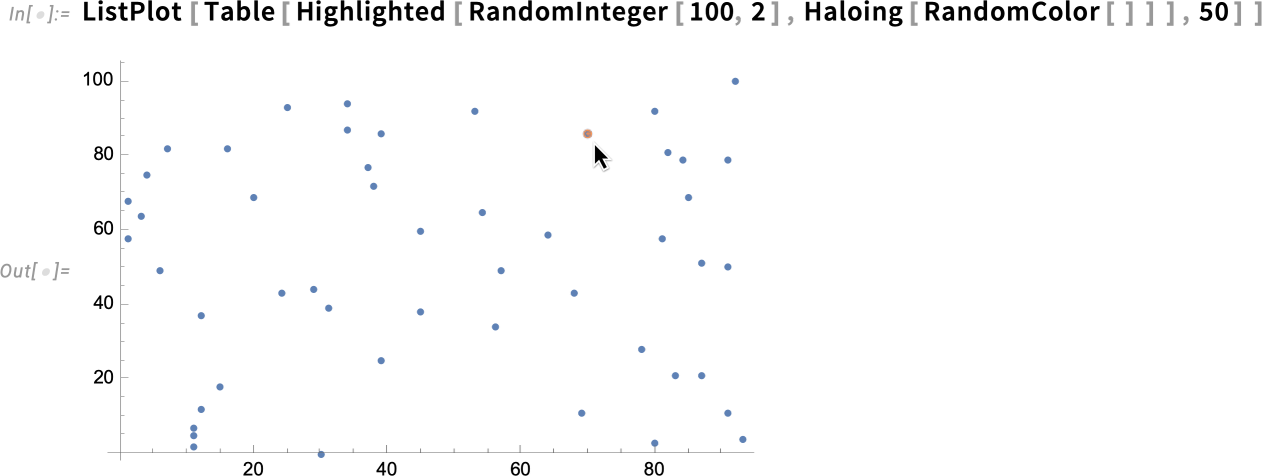
The same thing works for ListPlot:
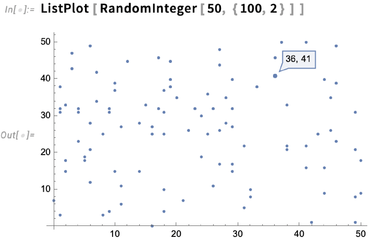
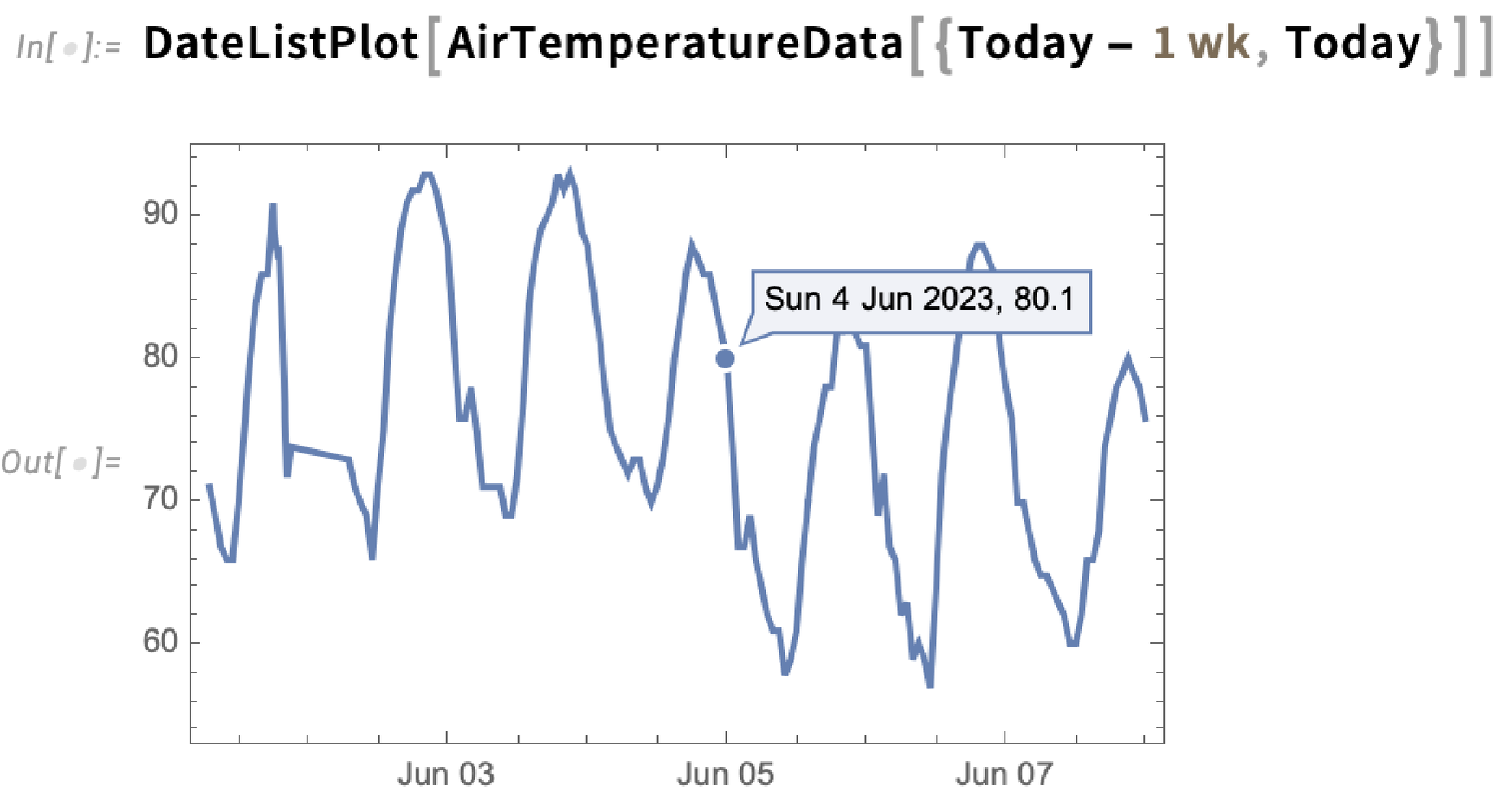
The highlighting can, for example, show dates too:
There are many choices for how the highlighting should be done. The simplest thing is just to specify a style in which to highlight whole curves:
But there are many other built-in highlighting specifications. Here, for example, is "XSlice":
In the end, though, highlighting is built up from a whole collection of components—like "NearestPoint", "Crosshairs", "XDropline", etc.—that you can assemble and style for yourself:
The option PlotHighlighting defines global highlighting in a plot. But by using the Highlighted “wrapper” you can specify that only a particular element in the plot should be highlighted:
For interactive and exploratory purposes, the kind of automatic highlighting we’ve just been showing is very convenient. But if you’re making a static presentation, you’ll need to “burn in” particular pieces of highlighting—which you can do with Placed:
In indicating elements in a graphic there are different effects one can use. In Version 13.1 we introduced DropShadowing[]. In Version 13.3 we’re introducing Haloing:
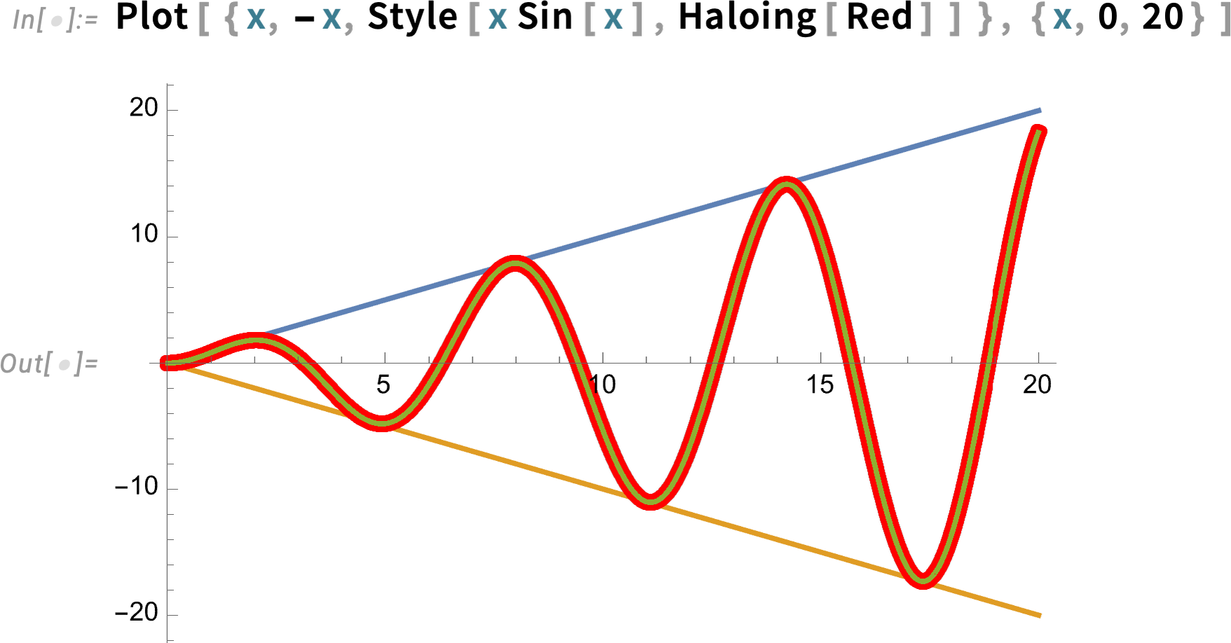
Haloing can also be combined with interactive highlighting:
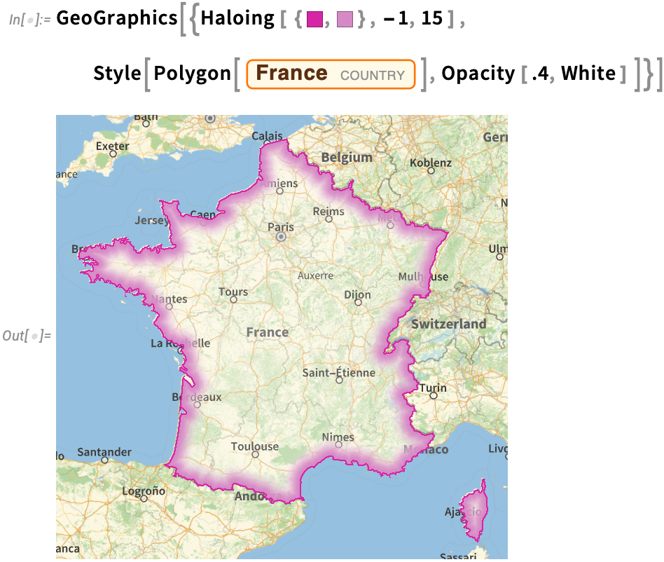
By the way, there are lots of nice effects you can get with Haloing in graphics. Here’s a geo example—including some parameters for the “orientation” and “thickness” of the haloing:
Publishing to Augmented + Virtual Reality
Throughout the history of the Wolfram Language 3D visualization has been an important capability. And we’re always looking for ways to share and communicate 3D geometry. Already back in the early 1990s we had experimental implementations of VR. But at the time there wasn’t anything like the kind of infrastructure for VR that would be needed to make this broadly useful. In the mid-2010s we then introduced VR functionality based on Unity—that provides powerful capabilities within the Unity ecosystem, but is not accessible outside.
Today, however, it seems there are finally broad standards emerging for AR and VR. And so in Version 13.3 we’re able to begin delivering what we hope will provide widely accessible AR and VR deployment from the Wolfram Language.
At a underlying level what we’re doing is to support the USD and GLTF geometry representation formats. But we’re also building a higher-level interface that allows anyone to “publish” 3D geometry for AR and VR.
Given a piece of geometry (which for now can’t involve too many polygons), all you do is apply ARPublish:

The result is a cloud object that has a certain underlying UUID, but is displayed in a notebook as a QR code. Now all you do is look at this QR code with your phone (or tablet, etc.) camera, and press the URL it extracts.
The result will be that the geometry you published with ARPublish now appears in AR on your phone:

Move your phone and you’ll see that your geometry has been realistically placed into the scene. You can also go to a VR “object” mode in which you can manipulate the geometry on your phone.
“Under the hood” there are some slightly elaborate things going on—particularly in providing the appropriate data to different kinds of phones. But the result is a first step in the process of easily being able to get AR and VR output from the Wolfram Language—deployed in whatever devices support AR and VR.
Getting the Details Right: The Continuing Story
In every version of Wolfram Language we add all sorts of fundamentally new capabilities. But we also work to fill in details of existing capabilities, continually pushing to make them as general, consistent and accurate as possible. In Version 13.3 there are many details that have been “made right”, in many different areas.
Here’s one example: the comparison (and sorting) of Around objects. Here are 10 random “numbers with uncertainty”:
These sort by their central value:
But if we look at these, many of their uncertainty regions overlap:

So when should we consider a particular number-with-uncertainty “greater than” another? In Version 13.3 we carefully take into account uncertainty when making comparisons. So, for example, this gives True:
But when there’s too big an uncertainty in the values, we no longer consider the ordering “certain enough”:
Here’s another example of consistency: the applicability of Duration. We introduced Duration to apply to explicit time constructs, things like Audio objects, etc. But in Version 13.3 it also applies to entities for which there’s a reasonable way to define a “duration”:


Dates (and times) are complicated things—and we’ve put a lot of effort into handling them correctly and consistently in the Wolfram Language. One concept that we introduced a few years ago is date granularity: the (subtle) analog of numerical precision for dates. But at first only some date functions supported granularity; now in Version 13.3 all date functions include a DateGranularity option—so that granularity can consistently be tracked through all date-related operations:

Also in dates, something that’s been added, particularly for astronomy, is the ability to deal with “years” specified by real numbers:

And one consequence of this is that it becomes easier to make a plot of something like astronomical distance as a function of time:

Also in astronomy, we’ve been steadily extending our capabilities to consistently fill in computations for more situations. In Version 13.3, for example, we can now compute sunrise, etc. not just from points on Earth, but from points anywhere in the solar system:

By the way, we’ve also made the computation of sunrise more precise. So now if you ask for the position of the Sun right at sunrise you’ll get a result like this:

How come the altitude of the Sun is not zero at sunrise? That’s because the disk of the Sun is of nonzero size, and “sunrise” is defined to be when any part of the Sun pokes over the horizon.
Even Easier to Type: Affordances for Wolfram Language Input
Back in 1988 when what’s now Wolfram Language first existed, the only way to type it was like ordinary text. But gradually we’ve introduced more and more “affordances” to make it easier and faster to type correct Wolfram Language input. In 1996, with Version 3, we introduced automatic spacing (and spanning) for operators, as well as brackets that flashed when they matched—and things like -> being automatically replaced by ![]() . Then in 2007, with Version 6, we introduced—with some trepidation at first—syntax coloring. We’d had a way to request autocompletion of a symbol name all the way back to the beginning, but it’d never been good or efficient enough for us to make it happen all the time as you type. But in 2012, for Version 9, we created a much more elaborate autocomplete system—that was useful and efficient enough that we turned it on for all notebook input. A key feature of this autocomplete system was its context-sensitive knowledge of the Wolfram Language, and how and where different symbols and strings typically appear. Over the past decade, we’ve gradually refined this system to the point where I, for one, deeply rely on it.
. Then in 2007, with Version 6, we introduced—with some trepidation at first—syntax coloring. We’d had a way to request autocompletion of a symbol name all the way back to the beginning, but it’d never been good or efficient enough for us to make it happen all the time as you type. But in 2012, for Version 9, we created a much more elaborate autocomplete system—that was useful and efficient enough that we turned it on for all notebook input. A key feature of this autocomplete system was its context-sensitive knowledge of the Wolfram Language, and how and where different symbols and strings typically appear. Over the past decade, we’ve gradually refined this system to the point where I, for one, deeply rely on it.
In recent versions, we’ve made other “typability” improvements. For example, in Version 12.3, we generalized the -> to ![]() transformation to a whole collection of “auto operator renderings”. Then in Version 13.0 we introduced “automatching” of brackets, in which, for example, if you enter [ at the end of what you’re typing, you’ll automatically get a matching ].
transformation to a whole collection of “auto operator renderings”. Then in Version 13.0 we introduced “automatching” of brackets, in which, for example, if you enter [ at the end of what you’re typing, you’ll automatically get a matching ].
Making “typing affordances” work smoothly is a painstaking and tricky business. But in every recent version we’ve steadily been adding more features that—in very “natural” ways—make it easier and faster to type Wolfram Language input.
In Version 13.3 one major change is an enhancement to autocompletion. Instead of just showing pure completions in which characters are appended to what’s already been typed, the autocompletion menu now includes “fuzzy completions” that fill in intermediate characters, change capitalization, etc.
So, for example, if you type “lp” you now get ListPlot as a completion (the little underlines indicate where the letters you actually type appear):

From a design point of view one thing that’s important about this is that it further removes the “short name” premium—and weights things even further on the side of wanting names that explain themselves when they’re read, rather than that are easy to type in an unassisted way. With the Wolfram Function Repository it’s become increasingly common to want to type ResourceFunction. And we’d been thinking that perhaps we should have a special, short notation for that. But with the new autocompletion, one can operationally just press three

When one designs something and gets the design right, people usually don’t notice; things just “work as they expect”. But when there’s a design error, that’s when people notice—and are frustrated by—the design. But then there’s another case: a situation where, for example, there are two things that could happen, and sometimes one wants one, and sometimes the other. In doing the design, one has to pick a particular branch. And when this happens to be the branch people want, they don’t notice, and they’re happy. But if they want the other branch, it can be confusing and frustrating.
In the design of the Wolfram Language one of the things that has to be chosen is the precedence for every operator: a + b × c means a + (b × c) because × has higher precedence than +. Often the correct order of precedences is fairly obvious. But sometimes it’s simply impossible to make everyone happy all the time. And so it is with ![]() and &. It’s very convenient to be able to add & at the end of something you type, and make it into a pure function. But that means if you type
and &. It’s very convenient to be able to add & at the end of something you type, and make it into a pure function. But that means if you type ![]() b &
b &![]() b &. When functions have options, however, one often wants things like name
b &. When functions have options, however, one often wants things like name ![]() function. The natural tendency is to type this as name
function. The natural tendency is to type this as name ![]() body &. But this will mean (name
body &. But this will mean (name ![]() body) & rather than name
body) & rather than name ![]() (body &). And, yes, when you try to run the function, it’ll notice it doesn’t have correct arguments and options specified. But you’d like to know that what you’re typing isn’t right as soon as you type it. And now in Version 13.3 we have a mechanism for that. As soon as you enter & to “end a function”, you’ll see the extent of the function flash:
(body &). And, yes, when you try to run the function, it’ll notice it doesn’t have correct arguments and options specified. But you’d like to know that what you’re typing isn’t right as soon as you type it. And now in Version 13.3 we have a mechanism for that. As soon as you enter & to “end a function”, you’ll see the extent of the function flash:
And, yup, you can see that’s wrong. Which gives you the chance to fix it as:
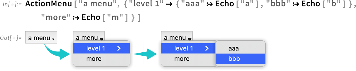
There’s another notebook-related update in Version 13.3 that isn’t directly related to typing, but will help in the construction of easy-to-navigate user interfaces. We’ve had ActionMenu since 2007—but it’s only been able to create one-level menus. In Version 13.3 it’s been extended to arbitrary hierarchical menus:
Again not directly related to typing, but now relevant to managing and editing code, there’s an update in Version 13.3 to package editing in the notebook interface. Bring up a .wl file and it’ll appear as a notebook. But its default toolbar is different from the usual notebook toolbar (and is newly designed in Version 13.3):

Go To now gives you a way to immediately go to the definition of any function whose name matches what you type, as well as any section, etc.:

The numbers on the right here are code line numbers; you can also go directly to a specific line number by typing :nnn.
The Elegant Code Project
One of the central goals—and achievements—of the Wolfram Language is to create a computational language that can be used not only as a way to tell computers what to do, but also as a way to communicate computational ideas for human consumption. In other words, Wolfram Language is intended not only to be written by humans (for consumption by computers), but also to be read by humans.
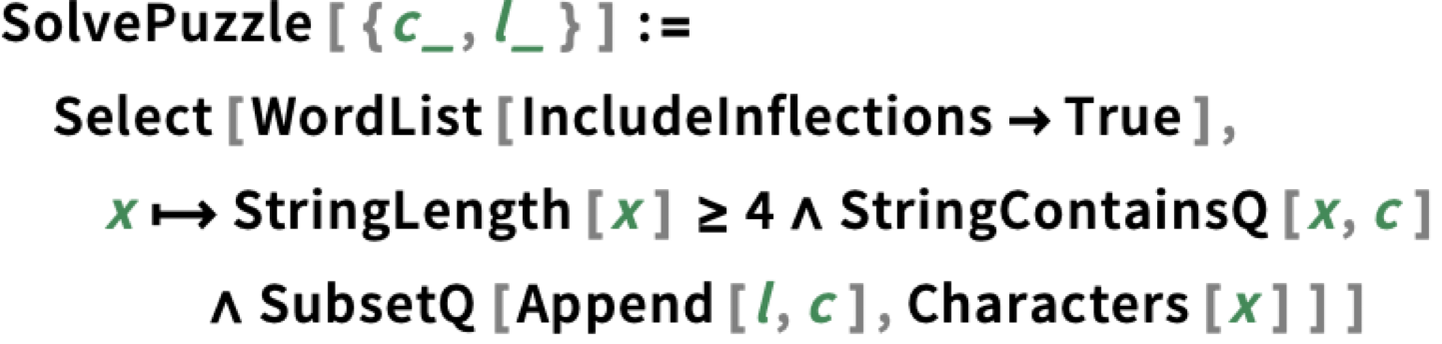
Crucial to this is the broad consistency of the Wolfram Language, as well as its use of carefully chosen natural-language-based names for functions, etc. But what can we do to make Wolfram Language as easy and pleasant as possible to read? In the past we’ve balanced our optimization of the appearance of Wolfram Language between reading and writing. But in Version 13.3 we’ve got the beginnings of our Elegant Code project—to find ways to render Wolfram Language to be specifically optimized for reading.
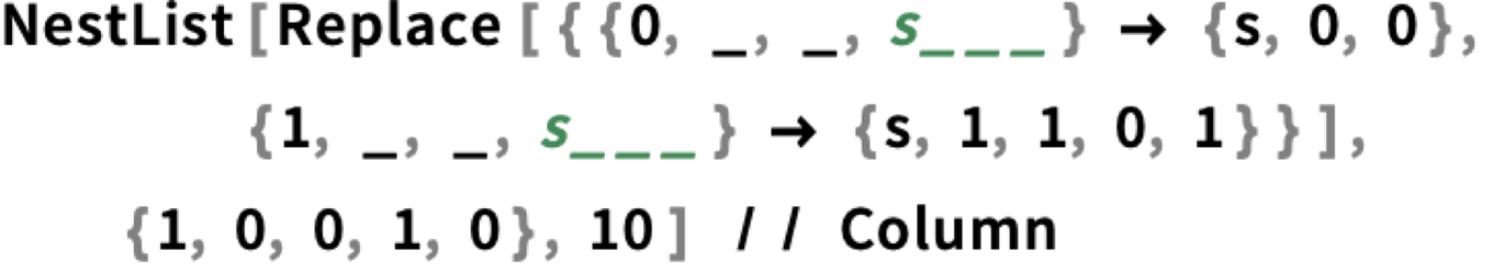
As an example, here’s a small piece of code (from my An Elementary Introduction to the Wolfram Language), shown in the default way it’s rendered in notebooks:
But in Version 13.3 you can use Format > Screen Environment > Elegant to set a notebook to use the current version of “elegant code”:
(And, yes, this is what we’re actually using for code in this post, as well as some other recent ones.) So what’s the difference? First of all, we’re using a proportionally spaced font that makes the names (here of symbols) easy to “read like words”. And second, we’re adding space between these “words”, and graying back “structural elements” like ![]() …
… ![]() and
and ![]() …
… ![]() . When you write a piece of code, things like these structural elements need to stand out enough for you to “see they’re right”. But when you’re reading code, you don’t need to pay as much attention to them. Because the Wolfram Language is so based on “word-like” names, you can typically “understand what it’s saying” just by “reading these words”.
. When you write a piece of code, things like these structural elements need to stand out enough for you to “see they’re right”. But when you’re reading code, you don’t need to pay as much attention to them. Because the Wolfram Language is so based on “word-like” names, you can typically “understand what it’s saying” just by “reading these words”.
Of course, making code “elegant” is not just a question of formatting; it’s also a question of what’s actually in the code. And, yes, as with writing text, it takes effort to craft code that “expresses itself elegantly”. But the good news is that the Wolfram Language—through its uniquely broad and high-level character—makes it surprisingly straightforward to create code that expresses itself extremely elegantly.
But the point now is to make that code not only elegant in content, but also elegant in formatting. In technical documents it’s common to see math that’s at least formatted elegantly. But when one sees code, more often than not, it looks like something only a machine could appreciate. Of course, if the code is in a traditional programming language, it’ll usually be long and not really intended for human consumption. But what if it’s elegantly crafted Wolfram Language code? Well then we’d like it to look as attractive as text and math. And that’s the point of our Elegant Code project.
There are many tradeoffs, and many issues to be navigated. But in Version 13.3 we’re definitely making progress. Here’s an example that doesn’t have so many “words”, but where the elegant code formatting still makes the “blocking” of the code more obvious:
Here’s a slightly longer piece of code, where again the elegant code formatting helps pull out “readable” words, as well as making the overall structure of the code more obvious:
Particularly in recent years, we’ve added many mechanisms to let one write Wolfram Language that’s easier to read. There are the auto operator renderings, like m[[i]] turning into ![]() . And then there are things like the
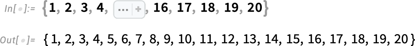
. And then there are things like the ![]() notation for pure functions. One particularly important element is Iconize, which lets you show any piece of Wolfram Language input in a visually “iconized” form—which nevertheless evaluates just like the corresponding underlying expression:
notation for pure functions. One particularly important element is Iconize, which lets you show any piece of Wolfram Language input in a visually “iconized” form—which nevertheless evaluates just like the corresponding underlying expression:
Iconize lets you effectively hide details (like large amounts of data, option settings, etc.) But sometimes you want to highlight things. You can do it with Style, Framed, Highlighted—and in Version 13.3, Squiggled:
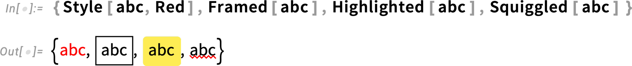
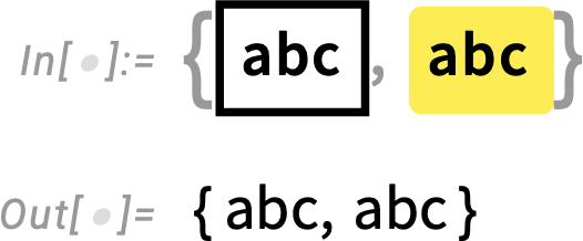
By default, all these constructs persist through evaluation. But in Version 13.3 all of them now have the option StripOnInput, and with this set, you have something that shows up highlighted in an input cell, but where the highlighting is stripped when the expression is actually fed to the Wolfram Language kernel.
These show their highlighting in the notebook:

But when used in input, the highlighting is stripped:
See More Also…
A great strength of the Wolfram Language (yes, perhaps initiated by my original 1988 Mathematica Book) is its detailed documentation—which has now proved valuable not only for human users but also for AIs. Plotting the number of words that appear in the documentation in successive versions, we see a strong progressive increase:

But with all that documentation, and all those new things to be documented, the problem of appropriately crosslinking everything has increased. Even back in Version 1.0, when the documentation was a physical book, there were “See Also’s” between functions:

And by now there’s a complicated network of such See Also’s:

But that’s just the network of how functions point to functions. What about other kinds of constructs? Like formats, characters or entity types—or, for that matter, entries in the Wolfram Function Repository, Wolfram Data Repository, etc. Well, in Version 13.3 we’ve done a first iteration of crosslinking all these kinds of things.
So here now are the “See Also” areas for Graph and Molecule:


Not only are there functions here; there are also other kinds of things that a person (or AI) looking at these pages might find relevant.
It’s great to be able to follow links, but sometimes it’s better just to have material immediately accessible, without following a link. Back in Version 1.0 we made the decision that when a function inherits some of its options from a “base function” (say Plot from Graphics), we only need to explicitly list the non-inherited option values. At the time, this was a good way to save a little paper in the printed book. But now the optimization is different, and finally in Version 13.3 we have a way to show “All Options”—tucked away so it doesn’t distract from the typically-more-important non-inherited options.
Here’s the setup for Plot. First, the list of non-inherited option values:

Then, at the end of the Details section

which opens to:

Pictures from Words: Generative AI for Images
One of the remarkable things that’s emerged as a possibility from recent advances in AI and neural nets is the generation of images from textual descriptions. It’s not yet realistic to do this at all well on anything but a high-end (and typically server) GPU-enabled machine. But in Version 13.3 there’s now a built-in function ImageSynthesize that can get images synthesized, for now through an external API.
You give text, and ImageSynthesize will try to generate images for which that text is a description:

Sometimes these images will be directly useful in their own right, perhaps as “theming images” for documents or user interfaces. Sometimes they will provide raw material that can be developed into icons or other art. And sometimes they are most useful as inputs to tests or other algorithms.
And one of the important things about ImageSynthesize is that it can immediately be used as part of any Wolfram Language workflow. Pick a random sentence from Alice in Wonderland:

Now ImageSynthesize can “illustrate” it:

Or we can get AI to feed AI:

ImageSynthesize is set up to automatically be able to synthesize images of different sizes:

You can take the output of ImageSynthesize and immediately process it:

ImageSynthesize can not only produce complete images, but can also fill in transparent parts of “incomplete” images:

In addition to ImageSynthesize and all its new LLM functionality, Version 13.3 also includes a number of advances in the core machine learning system for Wolfram Language. Probably the most notable are speedups of up to 10x and beyond for neural net training and evaluation on x86-compatible systems, as well as better models for ImageIdentify. There are also a variety of new networks in the Wolfram Neural Net Repository, particularly ones based on transformers.
Digital Twins: Fitting System Models to Data
It’s been five years since we first began to introduce industrial-scale systems engineering capabilities in the Wolfram Language. The goal is to be able to compute with models of engineering and other systems that can be described by (potentially very large) collections of ordinary differential equations and their discrete analogs. Our separate Wolfram System Modeler product provides an IDE and GUI for graphically creating such models.
For the past five years we’ve been able to do high-efficiency simulation of these models from within the Wolfram Language. And over the past few years we’ve been adding all sorts of higher-level functionality for programmatically creating models, and for systematically analyzing their behavior. A major focus in recent versions has been the synthesis of control systems, and various forms of controllers.
Version 13.3 now tackles a different issue, which is the alignment of models with real-world systems. The idea is to have a model which contains certain parameters, and then to determine these parameters by essentially fitting the model’s behavior to observed behavior of a real-world system.
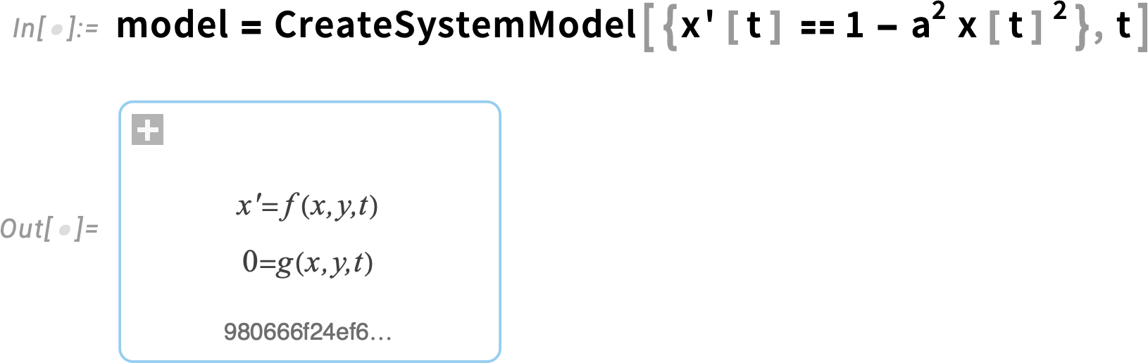
Let’s start by talking about a simple case where our model is just defined by a single ODE:
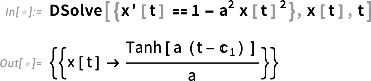
This ODE is simple enough that we can find its analytical solution:
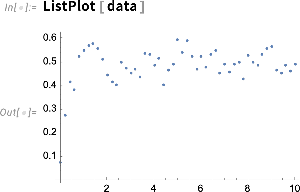
So now let’s make some “simulated real-world data” assuming
Here’s what the data looks like:
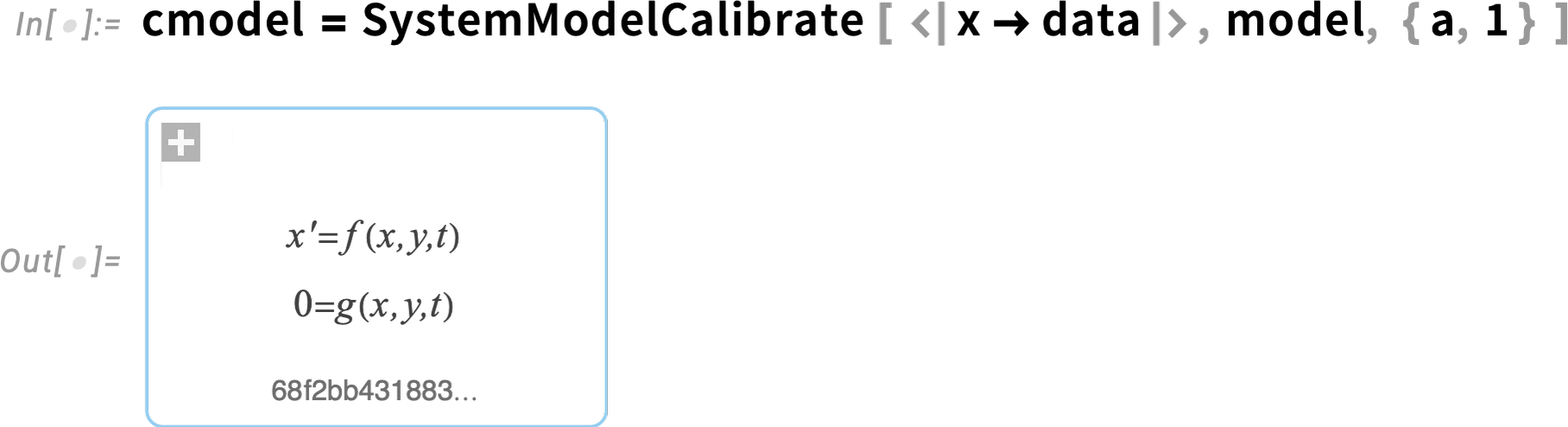
Now let’s try to “calibrate” our original model using this data. It’s a process similar to machine learning training. In this case we make an “initial guess” that the parameter a is 1; then when SystemModelCalibrate runs it shows the “loss” decreasing as the correct value of a is found:
The “calibrated” model does indeed have a ≈ 2:
Now we can compare the calibrated model with the data:
As a slightly more realistic engineering-style example let’s look at a model of an electric motor (with both electrical and mechanical parts):
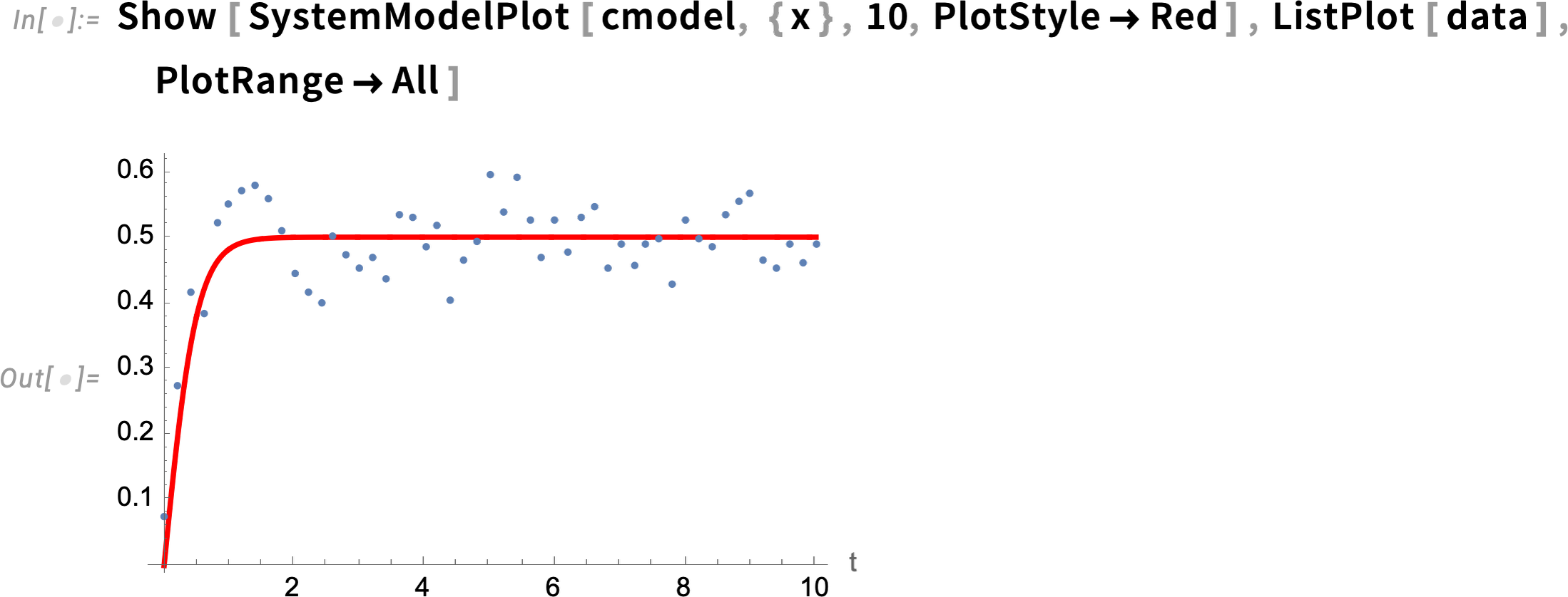
Let’s say we’ve got some data on the behavior of the motor; here we’ve assumed that we’ve measured the angular velocity of a component in the motor as a function of time. Now we can use this data to calibrate parameters of the model (here the resistance of a resistor and the damping constant of a damper):
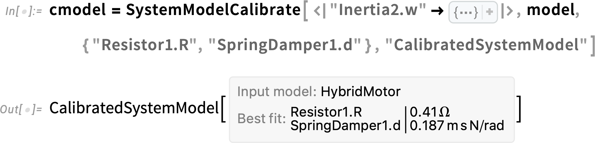
Here are the fitted parameter values:
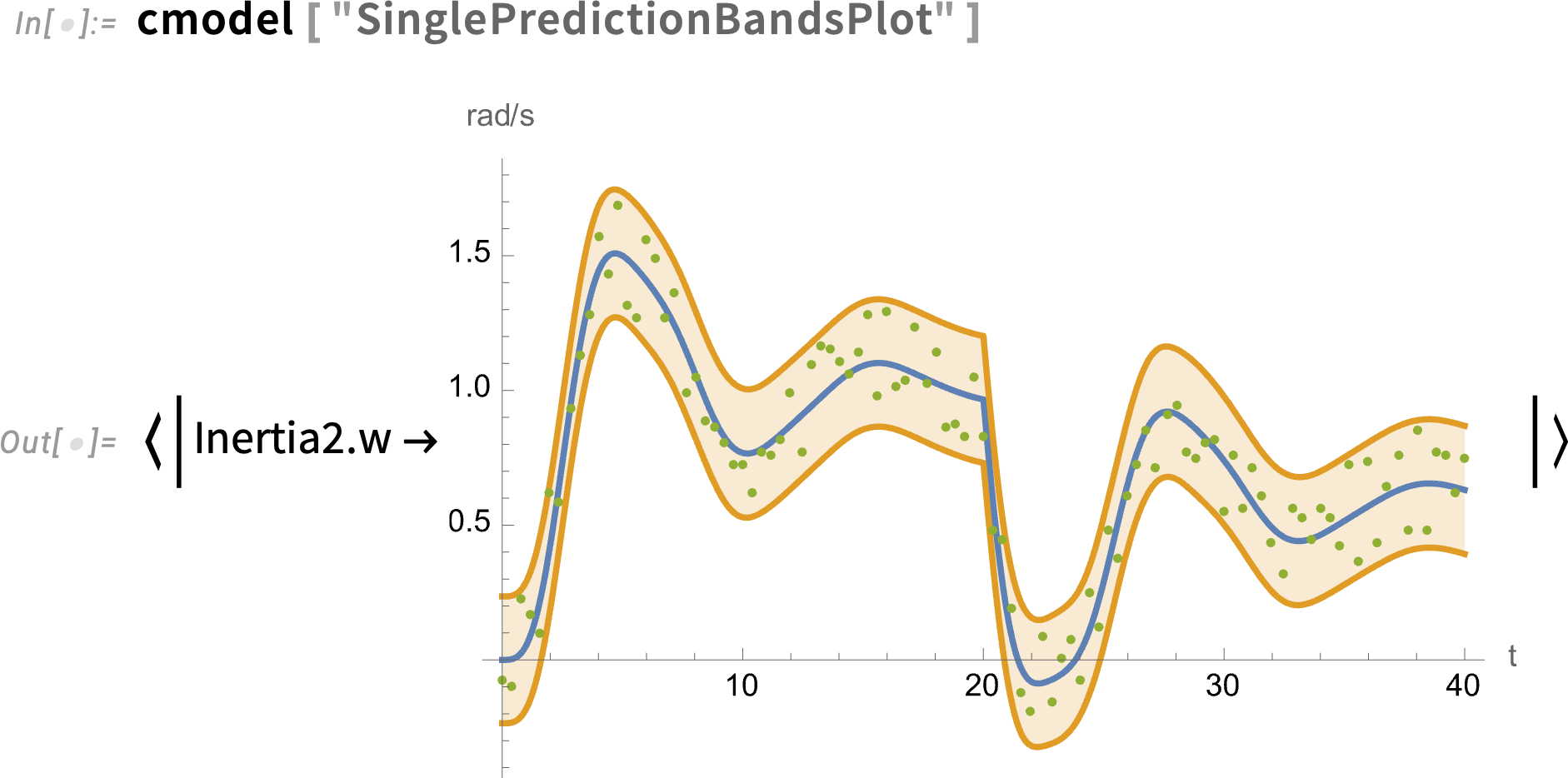
And here’s a full plot of the angular velocity data, together with the fitted model and its 95% confidence bands:
SystemModelCalibrate can be used not only in fitting a model to real-world data, but also for example in fitting simpler models to more complicated ones, making possible various forms of “model simplification”.
Symbolic Testing Framework
The Wolfram Language is by many measures one of the world’s most complex pieces of software engineering. And over the decades we’ve developed a large and powerful system for testing and validating it. A decade ago—in Version 10—we began to make some of our internal tools available for anyone writing Wolfram Language code. Now in Version 13.3 we’re introducing a more streamlined—and “symbolic”—version of our testing framework.
The basic idea is that each test is represented by a symbolic TestObject, created using TestCreate:

On its own, TestObject is an inert object. You can run the test it represents using TestEvaluate:

Each test object has a whole collection of properties, some of which only get filled in when the test is run:

It’s very convenient to have symbolic test objects that one can manipulate using standard Wolfram Language functions, say selecting tests with particular features, or generating new tests from old. And when one builds a test suite, one does it just by making a list of test objects.
This makes a list of test objects (and, yes, there’s some trickiness because TestCreate needs to keep unevaluated the expression that’s going to be tested):

But given these tests, we can now generate a report from running them:

TestReport has various options that allow you to monitor and control the running of a test suite. For example, here we’re saying to echo every "TestEvaluated" event that occurs:

Did You Get That Math Right?
Most of what the Wolfram Language is about is taking inputs from humans (as well as programs, and now AIs) and computing outputs from them. But a few years ago we started introducing capabilities for having the Wolfram Language ask questions of humans, and then assessing their answers.
In recent versions we’ve been building up sophisticated ways to construct and deploy “quizzes” and other collections of questions. But one of the core issues is always how to determine whether a person has answered a particular question correctly. Sometimes that’s easy to determine. If we ask “What is 2 + 2?”, the answer better be “4” (or conceivably “four”). But what if we ask a question where the answer is some algebraic expression? The issue is that there may be many mathematically equal forms of that expression. And it depends on what exactly one’s asking whether one considers a particular form to be the “right answer” or not.
For example, here we’re computing a derivative:
And here we’re doing a factoring problem:
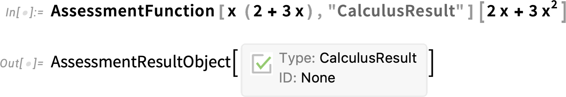
These two answers are mathematically equal. And they’d both be “reasonable answers” for the derivative if it appeared as a question in a calculus course. But in an algebra course, one wouldn’t want to consider the unfactored form a “correct answer” to the factoring problem, even though it’s “mathematically equal”.
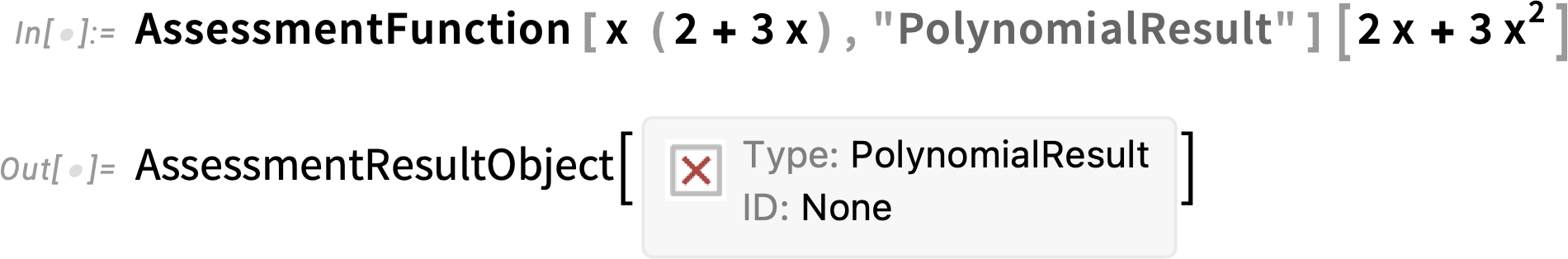
And to deal with these kinds of issues, we’re introducing in Version 13.3 more detailed mathematical assessment functions. With a "CalculusResult" assessment function, it’s OK to give the unfactored form:
But with a "PolynomialResult" assessment function, the algebraic form of the expression has to be the same for it to be considered “correct”:
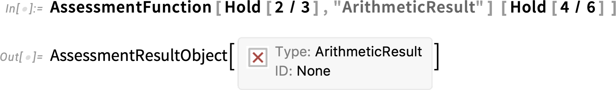
There’s also another type of assessment function—"ArithmeticResult"—which only allows trivial arithmetic rearrangements, so that it considers 2 + 3 equivalent to 3 + 2, but doesn’t consider 2/3 equivalent to 4/6:
Here’s how you’d build a question with this:
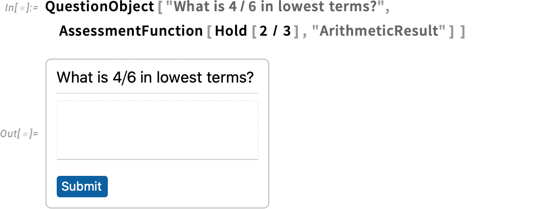
And now if you type “2/3” it’ll say you’ve got it right, but if you type “4/6” it won’t. However, if you use, say, "CalculusResult" in the assessment function, it’ll say you got it right even if you type “4/6”.
Streamlining Parallel Computation
Ever since the mid-1990s there’s been the capability to do parallel computation in the Wolfram Language. And certainly for me it’s been critical in a whole range of research projects I’ve done. I currently have 156 cores routinely available in my “home” setup, distributed across 6 machines. It’s sometimes challenging from a system administration point of view to keep all those machines and their networking running as one wants. And one of the things we’ve been doing in recent versions—and now completed in Version 13.3—is to make it easier from within the Wolfram Language to see and manage what’s going on.
It all comes down to specifying the configuration of kernels. And in Version 13.3 that’s now done using symbolic KernelConfiguration objects. Here’s an example of one:
There’s all sorts of information in the kernel configuration object:
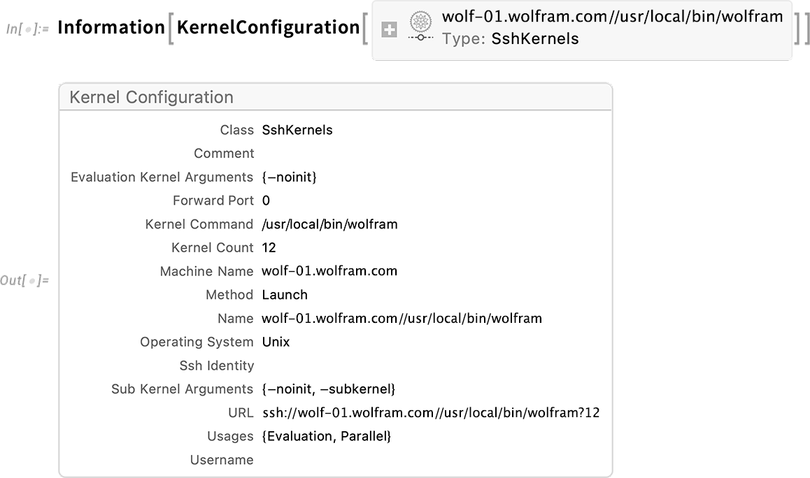
It describes “where” a kernel with that configuration will be, how to get to it, and how it should be launched. The kernel might just be local to your machine. Or it might be on a remote machine, accessible through ssh, or https, or our own wstp (Wolfram Symbolic Transport Protocol) or lwg (Lightweight Grid) protocols.
In Version 13.3 there’s now a GUI for setting up kernel configurations:

The Kernel Configuration Editor lets you enter all the details that are needed, about network connections, authentication, locations of executables, etc.
But once you’ve set up a KernelConfiguration object, that’s all you ever need—for example to say “where” to do a remote evaluation:
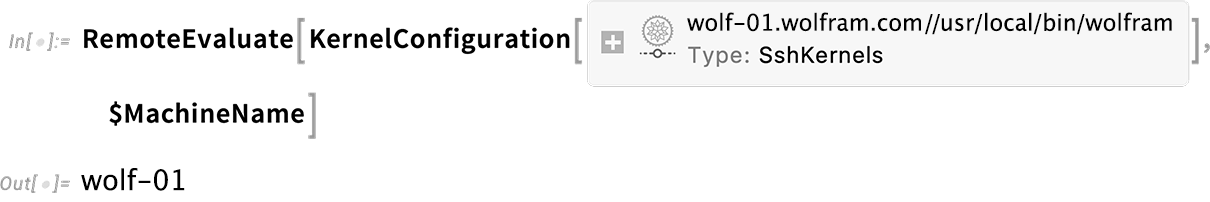
ParallelMap and other parallel functions then just work by doing their computations on kernels specified by a list of KernelConfiguration objects. You can set up the list in the Kernels Settings GUI:

Here’s my personal default collection of parallel kernels:
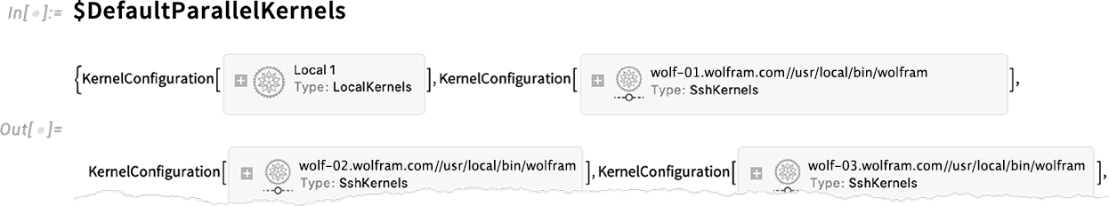
This now counts the number of individual kernels running on each machine specified by these configurations:
In Version 13.3 a convenient new feature is named collections of kernels. For example, this runs a single “representative” kernel on each distinct machine:
Just Call That C Function! Direct Access to External Libraries
Let’s say you’ve got an external library written in C—or in some other language that can compile to a C-compatible library. In Version 13.3 there’s now foreign function interface (FFI) capability that allows you to directly call any function in the external library just using Wolfram Language code.
Here’s a very trivial C function:
![]()
This function happens to be included in compiled form in the compilerDemoBase library that’s part of Wolfram Language documentation. Given this library, you can use ForeignFunctionLoad to load the library and create a Wolfram Language function that directly calls the C addone function. All you need do is specify the library and C function, and then give the type signature for the function:
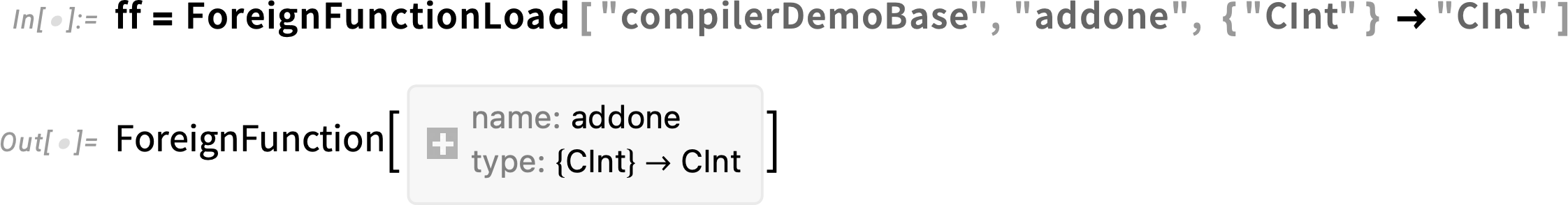
Now ff is a Wolfram Language function that calls the C addone function:
The C function addone happens to have a particularly simple type signature, that can immediately be represented in terms of compiler types that have direct analogs as Wolfram Language expressions. But in working with low-level languages, it’s very common to have to deal directly with raw memory, which is something that never happens when you’re purely working at the Wolfram Language level.
So, for example, in the OpenSSL library there’s a function called RAND_bytes, whose C type signature is:
![]()
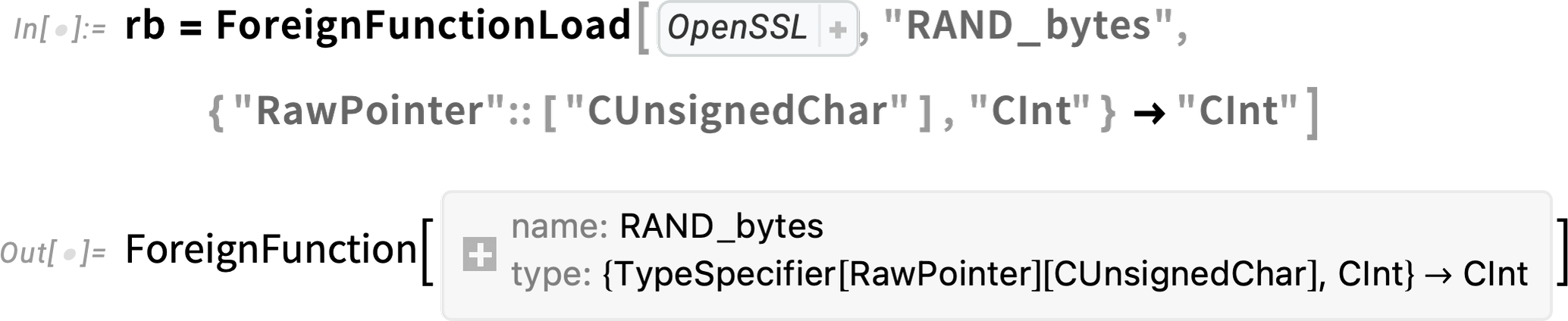
And the important thing to notice is that this contains a pointer to a buffer buf that gets filled by RAND_bytes. If you were calling RAND_bytes from C, you’d first allocate memory for this buffer, then—after calling RAND_bytes—read back whatever was written to the buffer. So how can you do something analogous when you’re calling RAND_bytes using ForeignFunction in Wolfram Language? In Version 13.3 we’re introducing a family of constructs for working with pointers and raw memory.
So, for example, here’s how we can create a Wolfram Language foreign function corresponding to RAND_bytes:
But to actually use this, we need to be able to allocate the buffer, which in Version 13.3 we can do with RawMemoryAllocate:
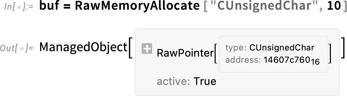
This creates a buffer that can store 10 unsigned chars. Now we can call rb, giving it this buffer:
rb will fill the buffer—and then we can import the results back into Wolfram Language:
There’s some complicated stuff going on here. RawMemoryAllocate does ultimately allocate raw memory—and you can see its hex address in the symbolic object that’s returned. But RawMemoryAllocate creates a ManagedObject, which keeps track of whether it’s being referenced, and automatically frees the memory that’s been allocated when nothing references it anymore.
Long ago languages like BASIC provided PEEK and POKE functions for reading and writing raw memory. It was always a dangerous thing to do—and it’s still dangerous. But it’s somewhat higher level in Wolfram Language, where in Version 13.3 there are now functions like RawMemoryRead and RawMemoryWrite. (For writing data into a buffer, RawMemoryExport is also relevant.)
Most of the time it’s very convenient to deal with memory-managed ManagedObject constructs. But for the full low-level experience, Version 13.3 provides UnmanageObject, which disconnects automatic memory management for a managed object, and requires you to explicitly use RawMemoryFree to free it.
One feature of C-like languages is the concept of a function pointer. And normally the function that the pointer is pointing to is just something like a C function. But in Version 13.3 there’s another possibility: it can be a function defined in Wolfram Language. Or, in other words, from within an external C function it’s possible to call back into the Wolfram Language.
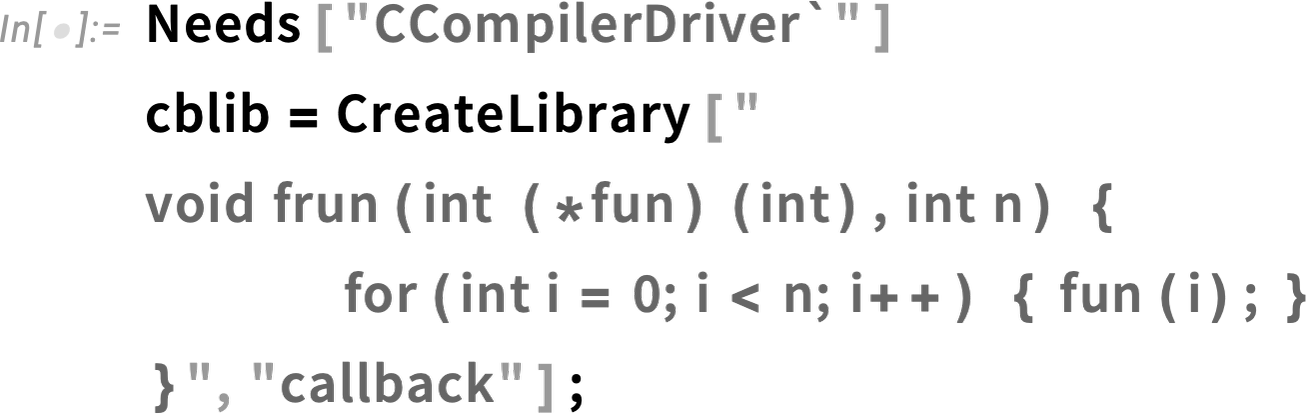
Let’s use this C program:
![]()
You can actually compile it right from Wolfram Language using:
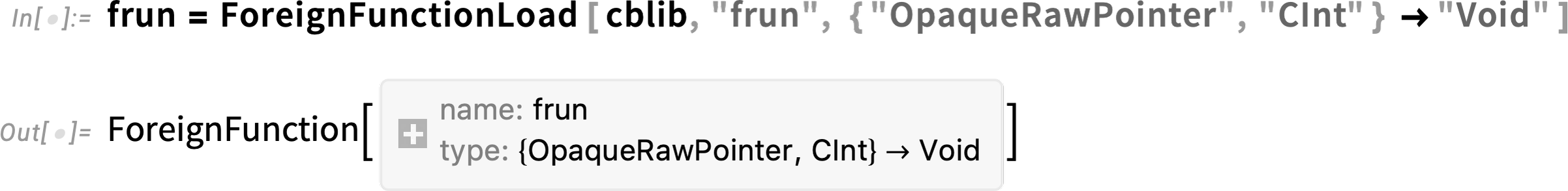
Now we load frun as a foreign function—with a type signature that uses "OpaqueRawPointer" to represent the function pointer:
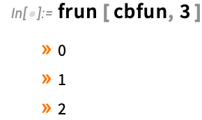
What we need next is to create a function pointer that points to a callback to Wolfram Language:
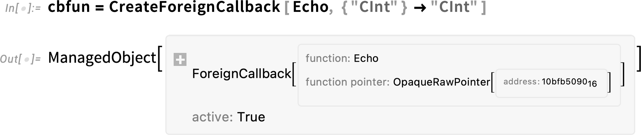
The Wolfram Language function here is just Echo. But when we call frun with the cbfun function pointer we can see our C code calling back into Wolfram Language to evaluate Echo:
ForeignFunctionLoad provides an extremely convenient way to call external C-like functions directly from top-level Wolfram Language. But if you’re calling C-like functions a great many times, you’ll sometimes want to do it using compiled Wolfram Language code. And you can do this using the LibraryFunctionDeclaration mechanism that was introduced in Version 13.1. It’ll be more complicated to set up, and it’ll require an explicit compilation step, but there’ll be slightly less “overhead” in calling the external functions.
The Advance of the Compiler Continues
For several years we’ve had an ambitious project to develop a large-scale compiler for the Wolfram Language. And in each successive version we’re further extending and enhancing the compiler. In Version 13.3 we’ve managed to compile more of the compiler itself (which, needless to say, is written in Wolfram Language)—thereby making the compiler more efficient in compiling code. We’ve also enhanced the performance of the code generated by the compiler—particularly by optimizing memory management done in the compiled code.
Over the past several versions we’ve been steadily making it possible to compile more and more of the Wolfram Language. But it’ll never make sense to compile everything—and in Version 13.3 we’re adding KernelEvaluate to make it more convenient to call back from compiled code to the Wolfram Language kernel.
Here’s an example:
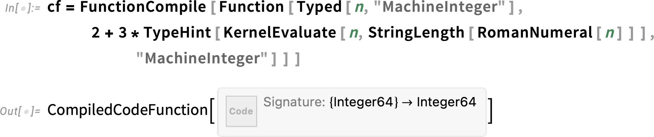
We’ve got an argument n that’s declared as being of type MachineInteger. Then we’re doing a computation on n in the kernel, and using TypeHint to specify that its result will be of type MachineInteger. There’s at least arithmetic going on outside the KernelEvaluate that can be compiled, even though the KernelEvaluate is just calling uncompiled code:
There are other enhancements to the compiler in Version 13.3 as well. For example, Cast now allows data types to be cast in a way that directly emulates what the C language does. There’s also now SequenceType, which is a type analogous to the Wolfram Language Sequence construct—and able to represent an arbitrary-length sequence of arguments to a function.
And Much More…
In addition to everything we’ve already discussed here, there are lots of other updates and enhancements in Version 13.3—as well as thousands of bug fixes.
Some of the additions fill out corners of functionality, adding completeness or consistency. Statistical fitting functions like LinearModelFit now accept input in all various association etc. forms that machine learning functions like Classify accept. TourVideo now lets you “tour” GeoGraphics, with waypoints specified by geo positions. ByteArray now supports the “corner case” of zero-length byte arrays. The compiler can now handle byte array functions, and additional string functions. Nearly 40 additional special functions can now handle numeric interval computations. BarcodeImage adds support for UPCE and Code93 barcodes. SolidMechanicsPDEComponent adds support for the Yeoh hyperelastic model. And—twenty years after we first introduced export of SVG, there’s now built-in support for import of SVG not only to raster graphics, but also to vector graphics.
There are new “utility” functions like RealValuedNumberQ and RealValuedNumericQ. There’s a new function FindImageShapes that begins the process of systematically finding geometrical forms in images. There are a number of new data structures—like "SortedKeyStore" and "CuckooFilter".
There are also functions whose algorithms—and output—have been improved. ImageSaliencyFilter now uses new machine-learning-based methods. RSolveValue gives cleaner and smaller results for the important case of linear difference equations with constant coefficients.