This Is a Big Release

Version 14.2 launched on January 23 of this year. Now, today, just over six months later, we’re launching Version 14.3. And despite its modest .x designation, it’s a big release, with lots of important new and updated functionality, particularly in core areas of the system.

I’m particularly pleased to be able to report that in this release we’re delivering an unusually large number of long-requested features. Why didn’t they come sooner? Well, they were hard—at least to build to our standards. But now they’re here, ready for everyone to use.

Those who’ve been following our livestreamed software design reviews (42 hours of them since Version 14.2) may get some sense of the effort we put into getting the design of things right. And in fact we’ve been consistently putting in that kind of effort now for nearly four decades—ever since we started developing Version 1.0. And the result is something that I think is completely unique in the software world—a system that is consistent and coherent through and through, and that has maintained compatibility for 37 years.

It’s a very big system now, and even I sometimes forget some of the amazing things it can do. But what now routinely helps me with that is our Notebook Assistant, released late last year. If I’m trying to figure out how to do something, I’ll just type some vague description of what I want into the Notebook Assistant. The Notebook Assistant is then remarkably good at “crispening up” what I’m asking, and producing relevant pieces of Wolfram Language code.

Often I was too vague for that code to be exactly what I want. But it almost always puts me on the right track, and with small modifications ends up being exactly what I need.

It’s a very good workflow, made possible by combining the latest AI with the unique characteristics of the Wolfram Language. I ask something vague. The Notebook Assistant gives me precise code. But the crucial thing is that the code isn’t programming language code, it’s Wolfram Language computational language code. It’s code that’s specifically intended to be read by humans and to represent the world computationally at as high a level as possible. The AI is going to behave in the kind of heuristic way that AIs do. But when you pick out the Wolfram Language code you want, you get something precise that you can build on, and rely on.

It’s amazing how important the design consistency of the Wolfram Language is in so many ways. It’s what allows the different facets of the language to interoperate so smoothly. It’s what makes it easy to learn new areas of the language. And, these days, it’s also what makes it easy for AIs to use the language well—calling on it as a tool much like humans do.

The fact that the Wolfram Language is so consistent in its design—and has so much built into it—has another consequence too: it means that it’s easy to add to it. And over the last 6 years, a rather staggering 3200+ add-on functions have been published in the Wolfram Function Repository. And, yes, quite a few of these functions may end up developing into full, built-in functions, though sometimes a decade or more hence. But here and now the Notebook Assistant knows about them in their current form—and can automatically show you where they might fit into things you’re doing.

OK, but let’s get back to Version 14.3. Where there’s a lot to talk about…

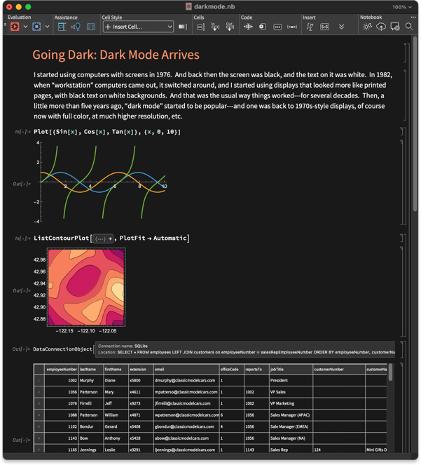
Going Dark: Dark Mode Arrives

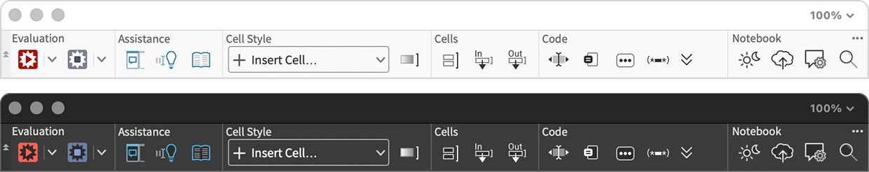
I started using computers with screens in 1976. And back then every screen was black, and the text on it was white. In 1982, when “workstation” computers came out, it switched around, and I started using displays that looked more like printed pages, with black text on white backgrounds. And that was the usual way things worked—for several decades. Then, a little more than five years ago, “dark mode” started to be popular—and one was back to 1970s-style displays, of course now with full color, at much higher resolution, etc. We’ve had “dark mode styles” available in notebooks for a long time. But now, in Version 14.3, we have full support for dark mode. And if you set your system to Dark Mode, in Version 14.3 all notebooks will by default automatically display in dark mode:

You might think: isn’t it kinda trivial to set up dark mode? Don’t you just have to change the background to black, and text to white? Well, actually, there’s a lot, lot more to it. And in the end it’s a rather complex user interface—and algorithmic—challenge, that I think we’ve now solved very nicely in Version 14.3.

Here’s a basic question: what should happen to a plot when you go to dark mode? You want the axes to flip to white, but you want the curves to keep their colors (otherwise, what would happen to text that refers to curves by color?). And that’s exactly what happens in Version 14.3:

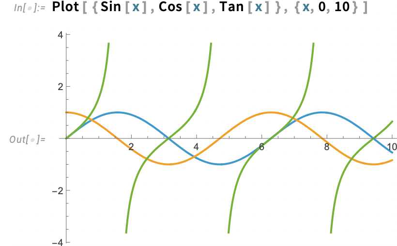
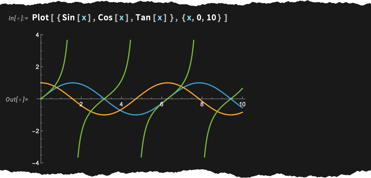
Needless to say, one tricky point is that the colors of the curves have to be chosen so they’ll look good in both light and dark mode. And actually in Version 14.2, when we “spiffed up” our default colors for plots, we did that in part precisely in anticipation of dark mode.

In Version 14.3 (as we’ll discuss below) we’ve continued spiffing up graphics colors, covering lots of tricky cases, and always setting things up to cover dark mode as well as light:

But graphics generated by computation aren’t the only kind of thing affected by dark mode. There are also, for example, endless user interface elements that all have to be adapted to look good in dark mode. In all, there are thousands of colors affected, all needing to be dealt with in a consistent and aesthetic way. And to do this, we’ve ended up inventing a whole range of methods and algorithms (which we’ll eventually make externally available as a paclet).

And the result, for example, is that something like the notebook can essentially automatically be configured to work in dark mode:

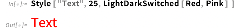
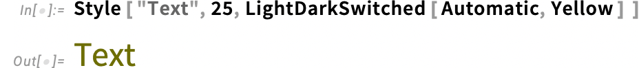
But what’s happening underneath? Needless to say, there’s a symbolic representation that’s involved. Normally, you specify a color as, for example, RGBColor[1,0,0]. But in Version 14.3, you can instead use a symbolic representation like:

In light mode, this will display as red; in dark mode, pink:

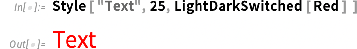
If you just give a single color in LightDarkSwitched, our automatic algorithms will be used, in this case producing in dark mode a pinkish color:

This specifies the dark mode color, automatically deducing an appropriate corresponding light mode color:

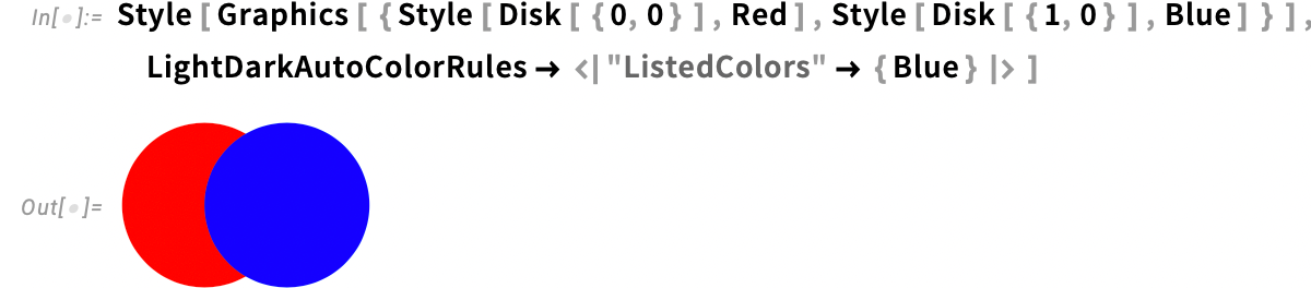
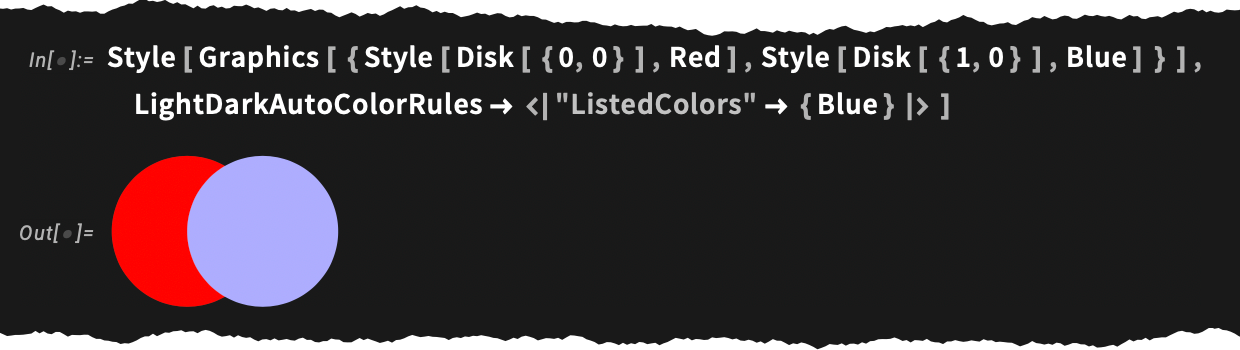
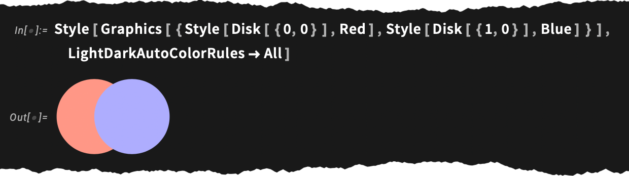
But what if you don’t want to explicitly insert LightDarkSwitched around every color you’re using? (For example, say you already have a large codebase full of colors.) Well, then you can use the new style option LightDarkAutoColorRules to specify more globally how you want to switch colors. So, for example, this says to do automatic light-dark switching for the “listed colors” (here just Blue) but not for others (e.g. Red):

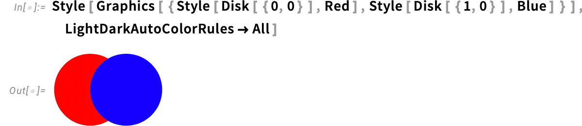
You can also use LightDarkAutoColorRules All which uses our automatic switching algorithms for all colors:

And then there’s the convenient LightDarkAutoColorRules "NonPlotColors" which says to do automatic switching, but only for colors that aren’t our default plot colors, which, as we discussed above, are set up to work unchanged in both light and dark mode.

There are many, many subtleties to all this. As one example, in Version 14.3 we’ve updated many functions to produce light-dark switched colors. But if those colors were stored in a notebook using LightDarkSwitched, then if you took that notebook and tried to view it with an earlier version those colors wouldn’t show up (and you’d get error indications). (As it happens, we already quietly introduced LightDarkSwitched in Version 14.2, but in earlier versions you’d be out of luck.) So how did we deal with this backward compatibility for light-dark switched colors our functions produce? Well, we don’t in fact store these colors in notebook expressions using LightDarkSwitched. Instead, we just store the colors in ordinary RGBColor etc. form, but the actual r, g, b values are numbers that have their “switched versions” steganographically encoded in high-order digits. Earlier versions just read this as a single color, imperceptibly adjusted from what it usually is; Version 14.3 reads it as a light-dark switched color.

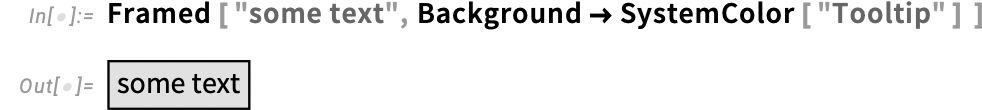
We’ve gone to a lot of effort to handle dark mode within our notebooks. But operating systems also have ways of handling dark mode. And sometimes you just want to have colors that follow the ones in your operating system. In Version 14.3 we’ve added SystemColor to do this. So, for example, here we say we want the background inside a frame to follow—in both light and dark mode—the color your operating system is using for tooltips:

One thing we haven’t explicitly mentioned yet is how textual content in notebooks is handled in dark mode. Black text is (obviously) rendered in white in dark mode. But what about section headings, or, for that matter, entities?

Well, they use different colors in light and dark mode. So how can you use those colors in your own programs? The answer is that you can use ThemeColor. ThemeColor is actually something we introduced in Version 14.2, but it’s part of a whole framework that we’re progressively building out in successive versions. And the idea is that ThemeColor allows you to access “theme colors” associated with particular “themes”. So, for example, there are "Accent1", etc. theme colors that—in a particular blend—are what’s used to get the color for the "Section" style. And with ThemeColor you can access these colors. So, for example, here is text in the "Accent3" theme color:

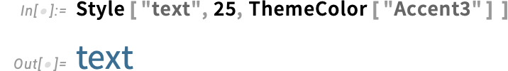
And, yes, it switches in dark mode:

Alright, so we’ve discussed all sorts of details of how light and dark mode work. But how do you determine whether a particular notebook should be in light or dark mode? Well, usually you don’t have to, because it’ll get switched automatically, following whatever your overall system settings are.

But if you want to explicitly lock in light or dark mode for a given notebook, you can do this with the button in the notebook toolbar. And you can also do this programmatically (or in the Wolfram System preferences) using the LightDark option.

So, OK, now we support dark mode. So… will I turn the clock back for myself by 45 years and return to using dark mode for most of my work (which, needless to say, is done in Wolfram Language)? Dark mode in Wolfram Notebooks looks so nice, I think I just might…

How Does It Relate to AI? Connecting with the Agentic World

In some ways the whole story of the Wolfram Language is about “AI”. It’s about automating as much as possible, so you (as a human) just have to “say what you want”, and then the system has a whole tower of automation that executes it for you. Of course, the big idea of the Wolfram Language is to provide the best way to “say what you want”—the best way to formalize your thoughts in computational terms, both so you can understand them better, and so your computer can go as far as it needs to work them out. Modern “post-ChatGPT” AI has been particularly important in adding a thicker “linguistic user interface” for all this. In Wolfram|Alpha we pioneered natural language understanding as a front end to computation; modern LLMs extend that to let you have whole conversations in natural language.

As I’ve discussed at some length elsewhere, what the LLMs are good at is rather different from what the Wolfram Language is good at. At some level LLMs can do the kinds of things unaided brains can also do (albeit sometimes on a larger scale, faster, etc.). But when it comes to raw computation (and precise knowledge) that’s not what LLMs (or brains) do well. But of course we know a very good solution to that: just have the LLM use Wolfram Language (and Wolfram|Alpha) as a tool. And indeed within a few months of the release of ChatGPT, we had set up ways to let LLMs call our technology as a tool. We’ve been developing ever better ways to have that happen—and indeed we’ll have a major release in this area soon.

It’s popular these days to talk about “AI agents” that “just go off and do useful things”. At some level the Wolfram Language (and Wolfram|Alpha) can be thought of as “universal agents”, able to do the full range of “computational things” (as well as having connectors to an immense number of external systems in the world). (Yes, Wolfram Language can send email, browse webpages— and “actuate” lots of other things in the world—and it’s been able to do these things for decades.) And if one builds the core of an agent out of LLMs, the Wolfram Language (and Wolfram|Alpha) serve as “universal tools” that the LLMs can call on.

So although LLMs and the Wolfram Language do very different kinds of things, we’ve been building progressively more elaborate ways for them to interact, and for one to be able to get the best from each of them. Back in mid-2023 we introduced LLMFunction, etc. as a way to call LLMs from within the Wolfram Language. Then we introduced LLMTool as a way to define Wolfram Language tools that LLMs can call. And in Version 14.3 we have another level in this integration: LLMGraph.

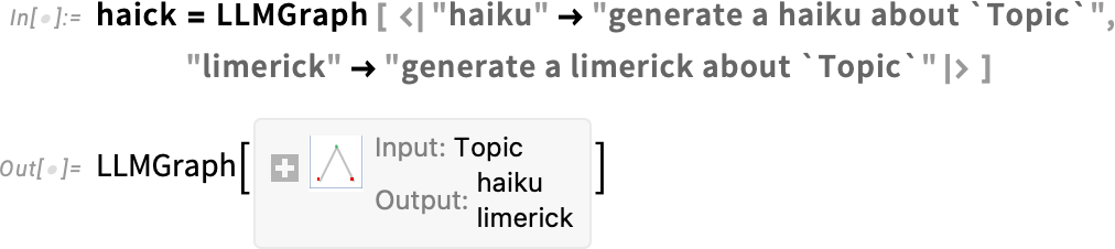
The goal of LLMGraph is to let you define an “agentic workflow” directly in Wolfram Language, specifying a kind of “plan graph” whose nodes can give either LLM prompts or Wolfram Language code to run. In effect, LLMGraph is a generalization of our existing LLM functions—with additional features such as the ability to run different parts in parallel, etc.

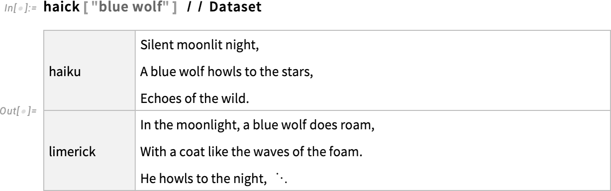
Here’s a very simple example: an LLMGraph that has just two nodes, which can be executed in parallel, one generating a haiku and one a limerick:

We can apply this to a particular input; the result is an association (which here we format with Dataset):

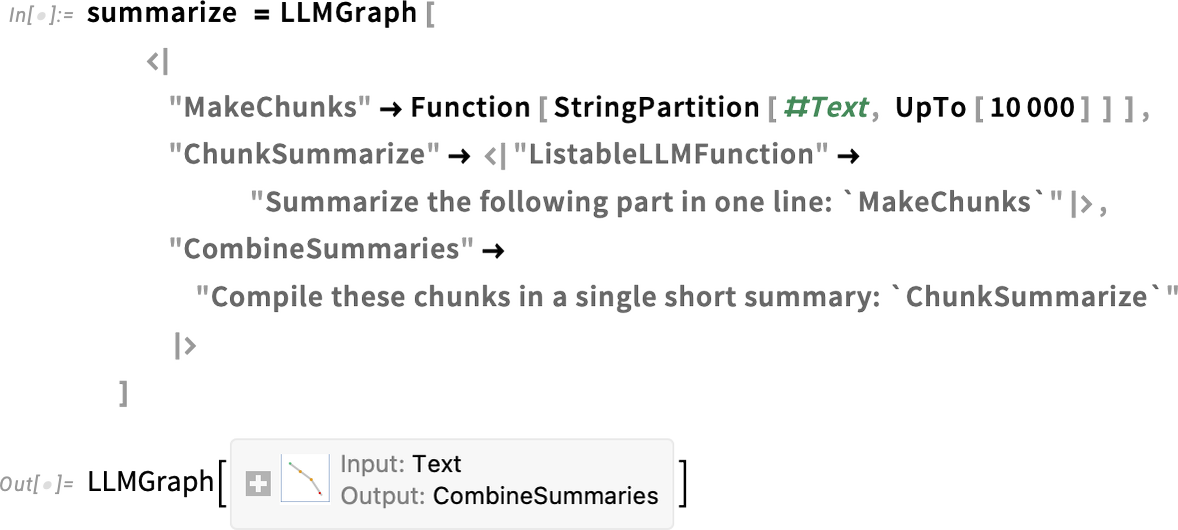
Here’s a slightly more complicated example—a workflow for summarizing text that breaks the text into chunks (using a Wolfram Language function) , then runs LLM functions in parallel to do the summarizing, then runs another LLM function to make a single summary from all the chunk summaries:

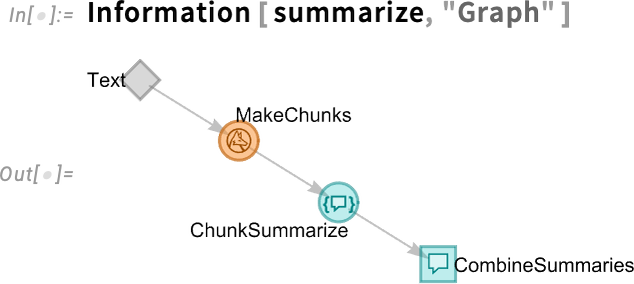
This visualizes our LLMGraph:

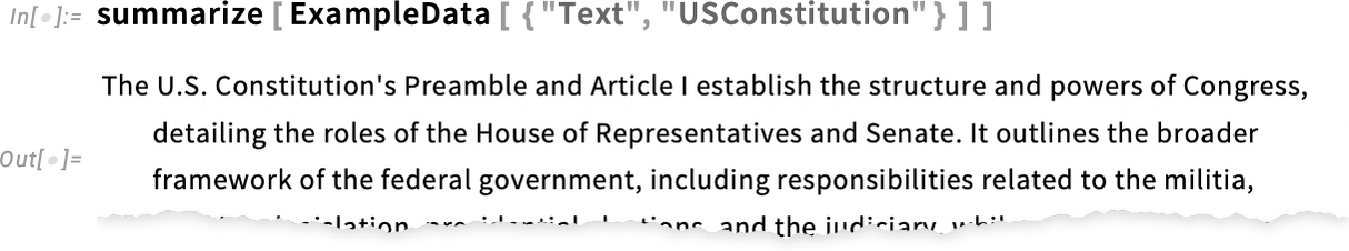
If we apply our LLMGraph, here to the US Constitution, we get a summary:

There are lots of detailed options for LLMGraph objects. Here, for example, for our "ChunkSummary" we used a "ListableLLMFunction" key, which specifies that the LLMFunction prompt we give can be threaded over a list of inputs (here the list of chunks generated by the Wolfram Language code in "TextChunk").

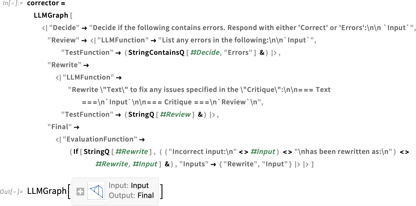
An important feature of LLMGraph is its support for “test functions”: nodes in the graph that do tests which determine whether another node needs to be run or not. Here’s a slightly more complicated example (and, yes, the LLM prompts are necessarily a bit verbose):

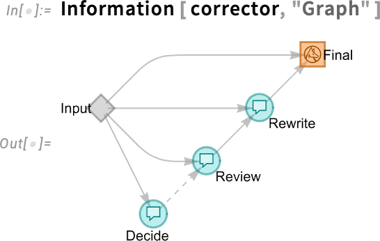
This visualizes the LLM graph:

Run it on a correct computation and it just returns the computation:

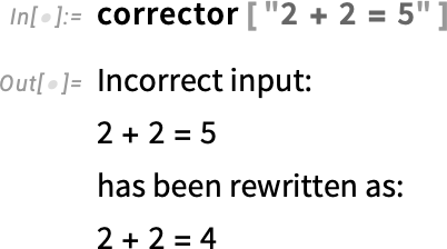
But run it on an incorrect computation and it’ll try to correct it, here correctly:

This is a fairly simple example. But—like everything in Wolfram Language—LLMGraph is built to scale up as far as you need. In effect, it provides a new way of programming—complete with asynchronous processing—for the “agentic” LLM world. Part of the ongoing integration of Wolfram Language and AI capabilities.

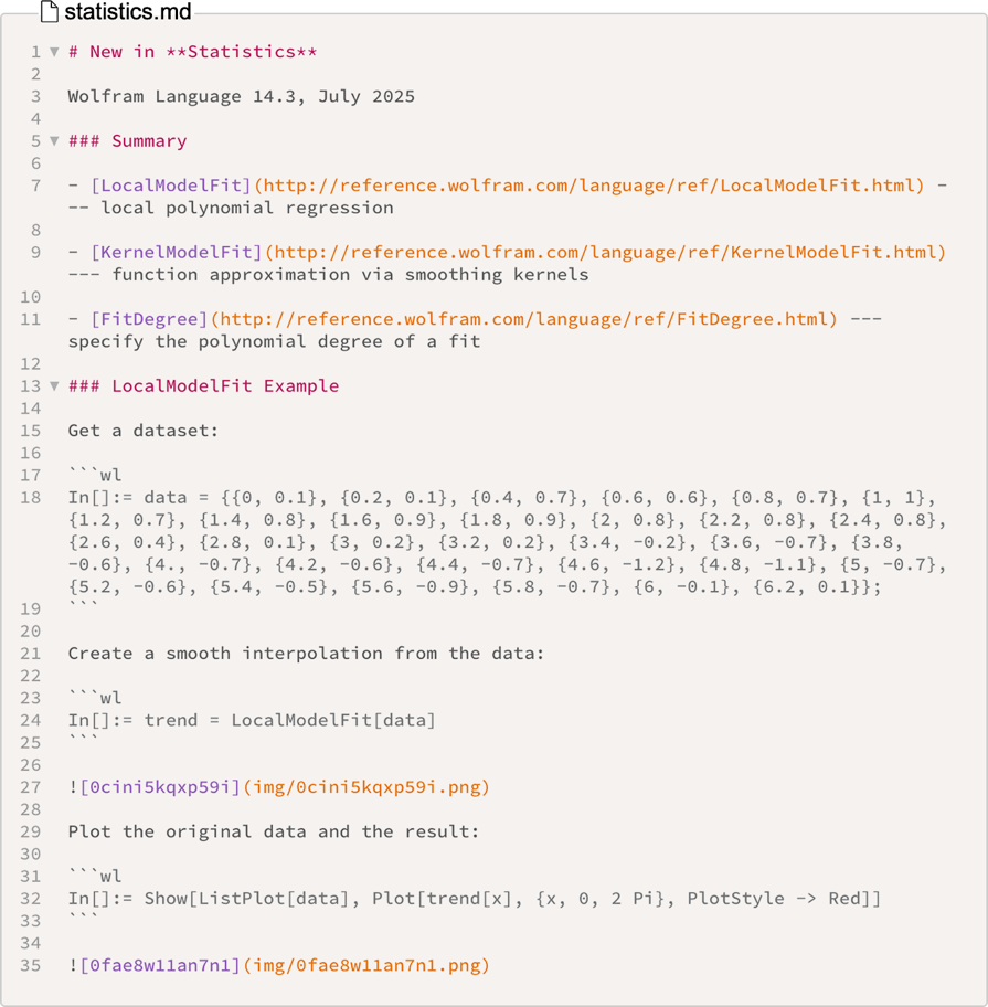
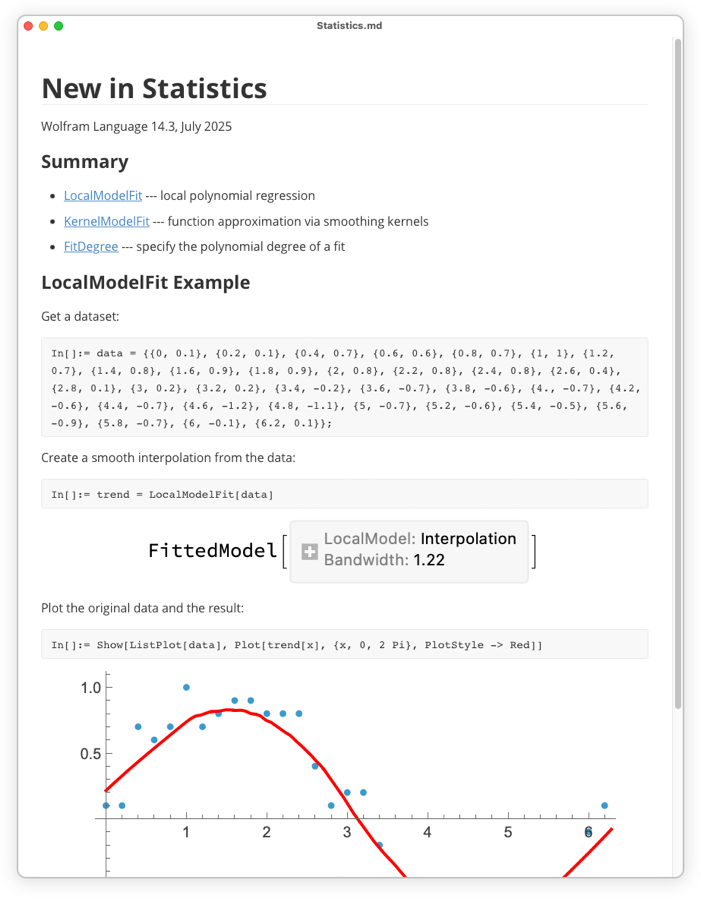
Just Put a Fit on That!

Let’s say you plot some data (and, yes, we’re using the new tabular data capabilities from Version 14.2):

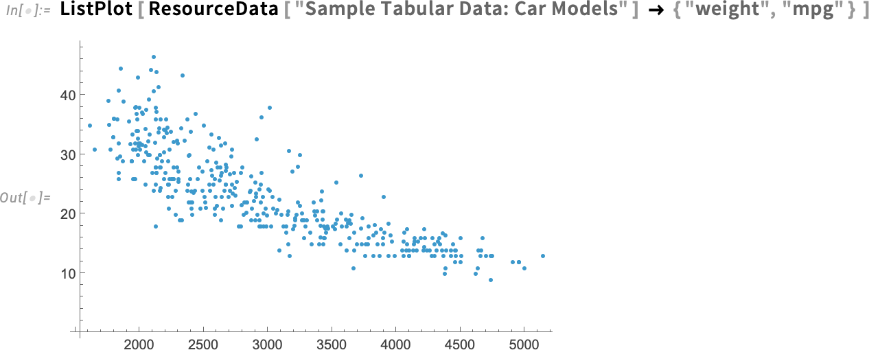
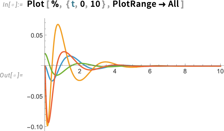
What’s really going on in this data? What are the trends? Often one finds oneself making some kind of fit to the data to try to find that out. Well, in Version 14.3 there’s now a very easy way to do that: ListFitPlot:

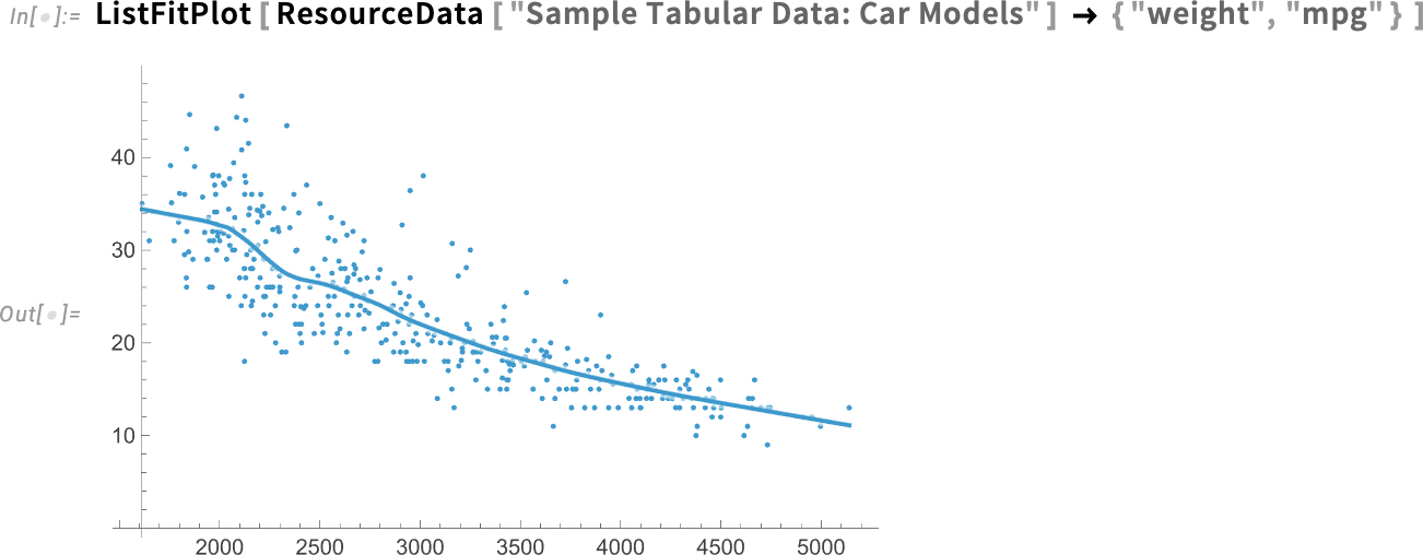
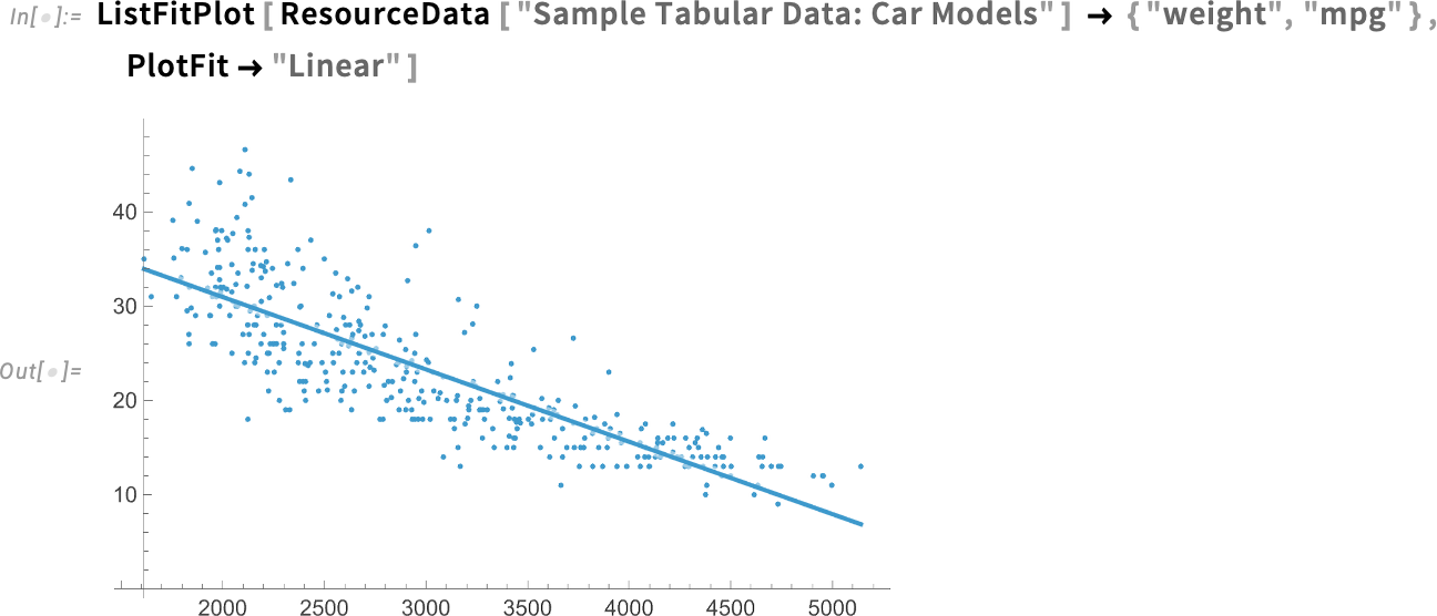
This is a local fit to the data (as we’ll discuss below). But what if we specifically want a global linear fit? There’s a simple option for that:

And here’s an exponential fit:

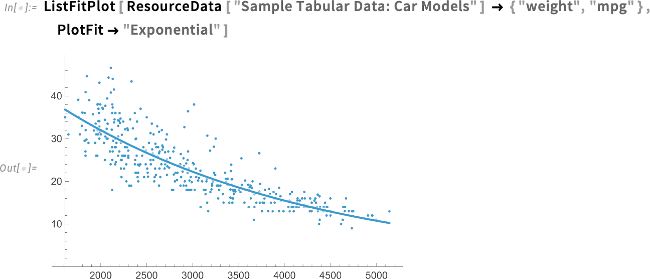
What we’re plotting here are the original data points together with the fit. The option PlotFitElements lets one select exactly what to plot. Like here we’re saying to also plot (95% confidence) band curves:

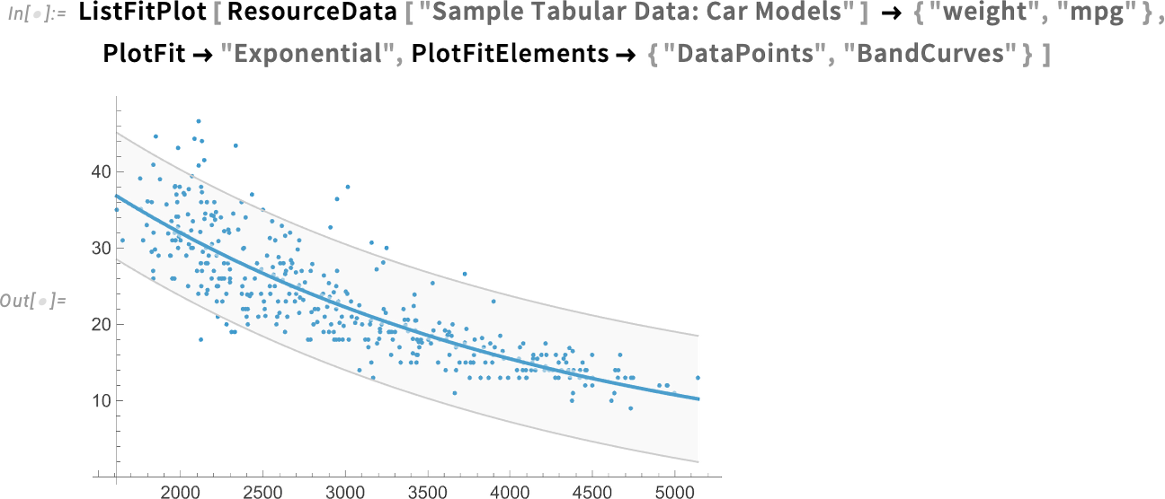
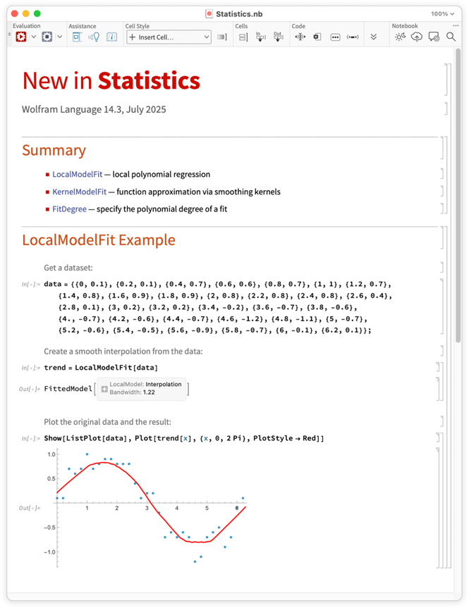
OK, so this is how one can visualize fits. But what about finding out what the fit actually was? Well, actually, we already had functions for doing that, like LinearModelFit and NonlinearModelFit. In Version 14.3, though, there’s also the new LocalModelFit:

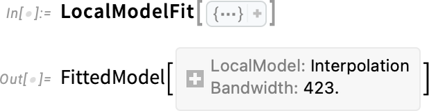
Like LinearModelFit etc. what this gives is a symbolic FittedModel object—which we can then, for example, plot:

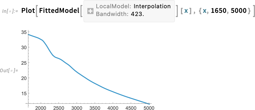
LocalModelFit is a non-parametric fitting function that works by doing local polynomial regressions (LOESS). Another new function in Version 14.3 is KernelModelFit, which fits to sums of basis function kernels:

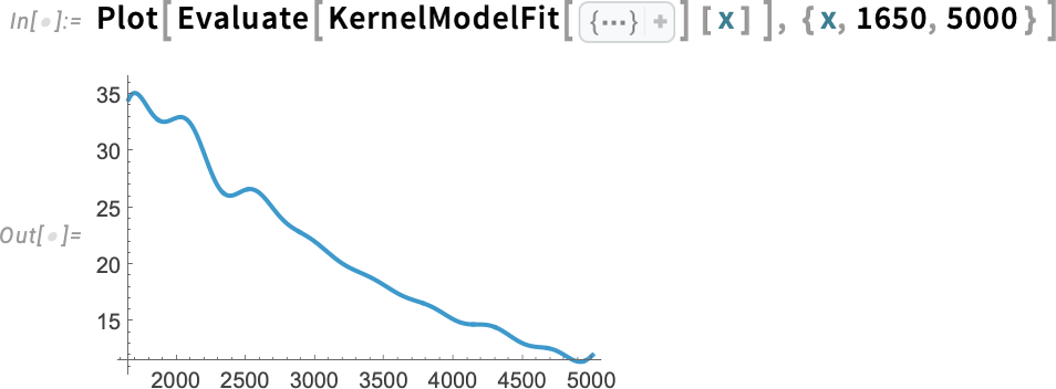
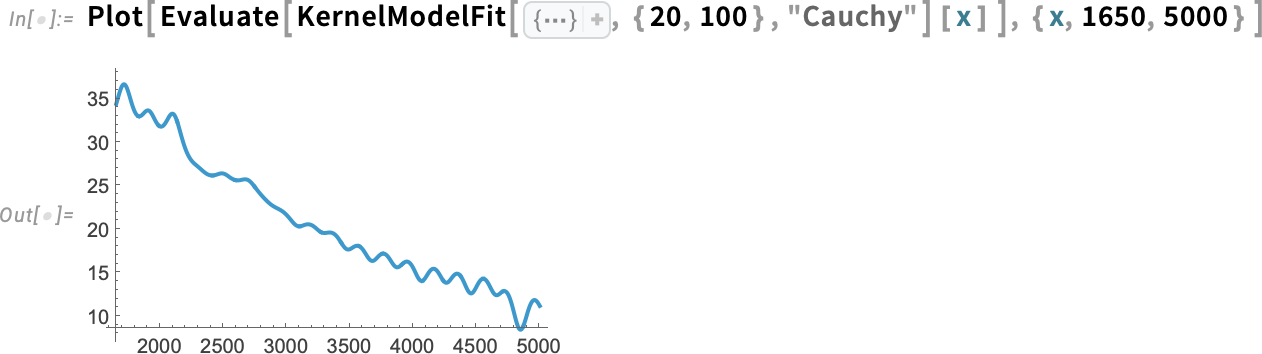
By default the kernels are Gaussian, and the number and width of them is chosen automatically. But here, for example, we’re asking for 20 Cauchy kernels with width 10:

What we just plotted is a best fit curve. But in Version 14.3 whenever we get a FittedModel we can ask not only for the best fit, but also for a fit with errors, represented by Around objects:

We can plot this to show the best fit, along with (95% confidence) band curves:

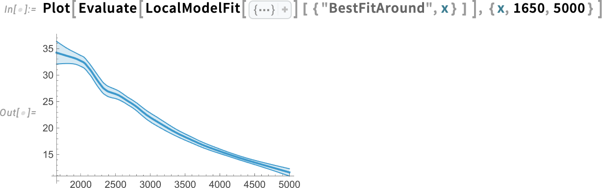
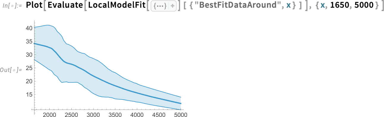
What this is showing is the best fit, together with the (“statistical”) uncertainty of the fit. Another thing you can do is to show band curves not for the fit, but for all the original data:

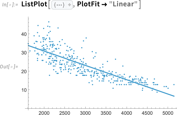
ListFitPlot is specifically set up to generate plots that show fits. As we just saw, you can also get such plots by first explicitly finding fits, and then plotting them. But there’s also another way to get plots that include fits, and that’s by adding the option PlotFit to “ordinary” plotting functions. It’s the very same PlotFit option that you can use in ListFitPlot to specify the type of fit to use. But in a function like ListPlot it specifies to add a fit:

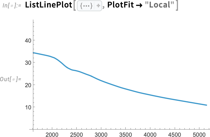
A function like ListLinePlot is set up to “draw a line through data”, and with PlotFit (like with InterpolationOrder) you can tell it “what line”. Here it’s a line based on a local model:

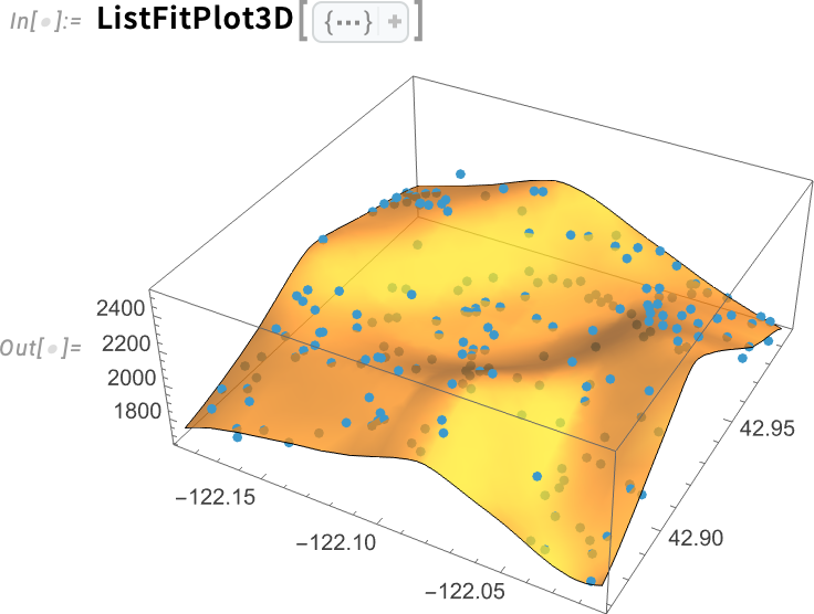
It’s also possible to do fits in 3D. And in Version 14.3, in analogy to ListFitPlot there’s also ListFitPlot3D, which fits a surface to a collection of 3D points:

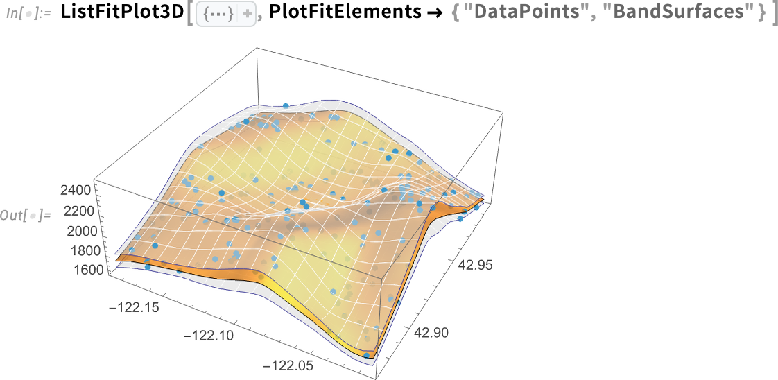
Here’s what happens if we include confidence band surfaces:

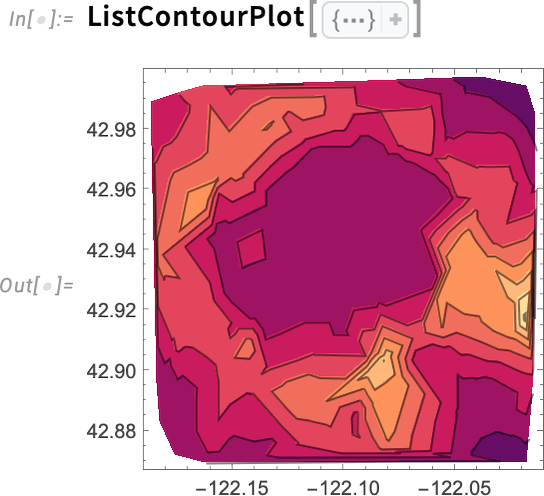
Functions like ListContourPlot also allow fits—and in fact it’s sometimes better to show only the fit for a contour plot. For example, here’s a “raw” contour plot:

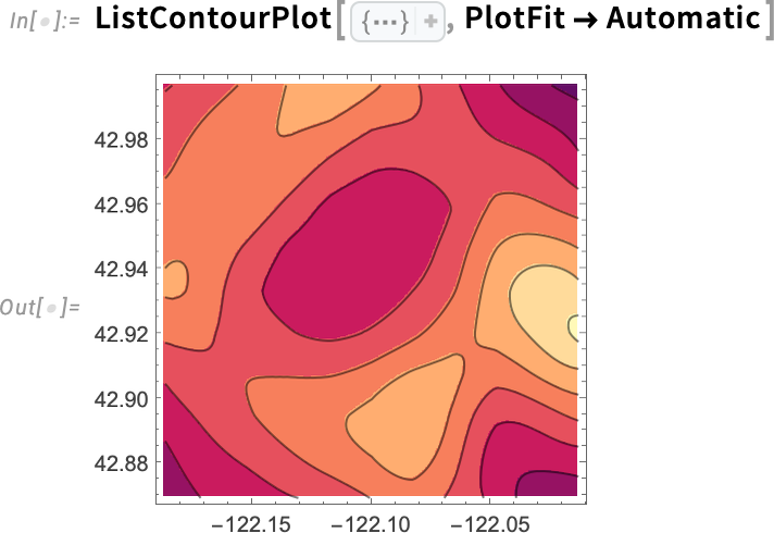
And here’s what we get if we plot not the raw data but a local model fit to the data:

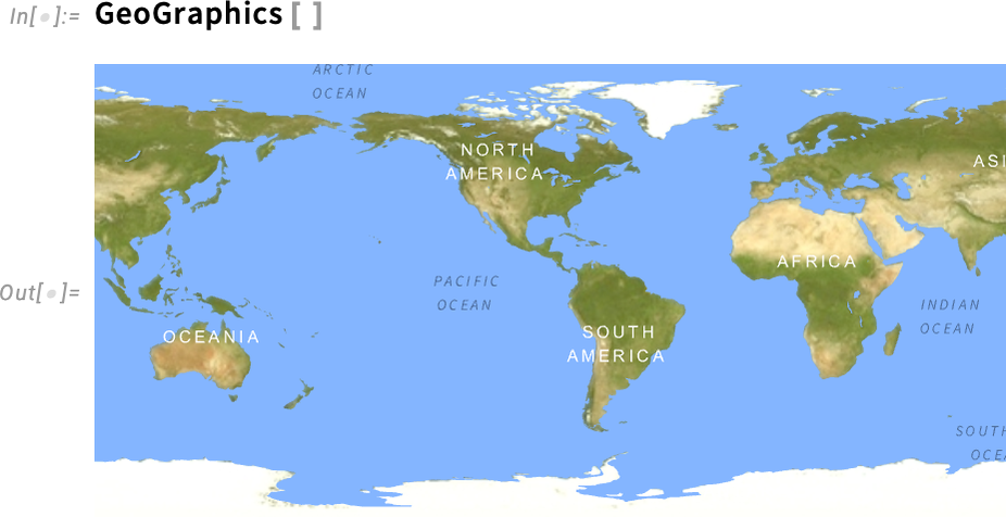
Maps Become More Beautiful

The world looks better now. Or, more specifically, in Version 14.3 we’ve updated the styles and rendering we’re using for maps:

Needless to say, this is yet another place where we have to deal with dark mode. Here’s the analogous image in dark mode:

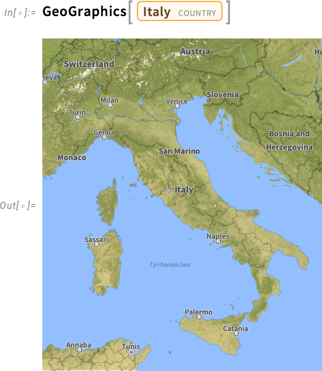
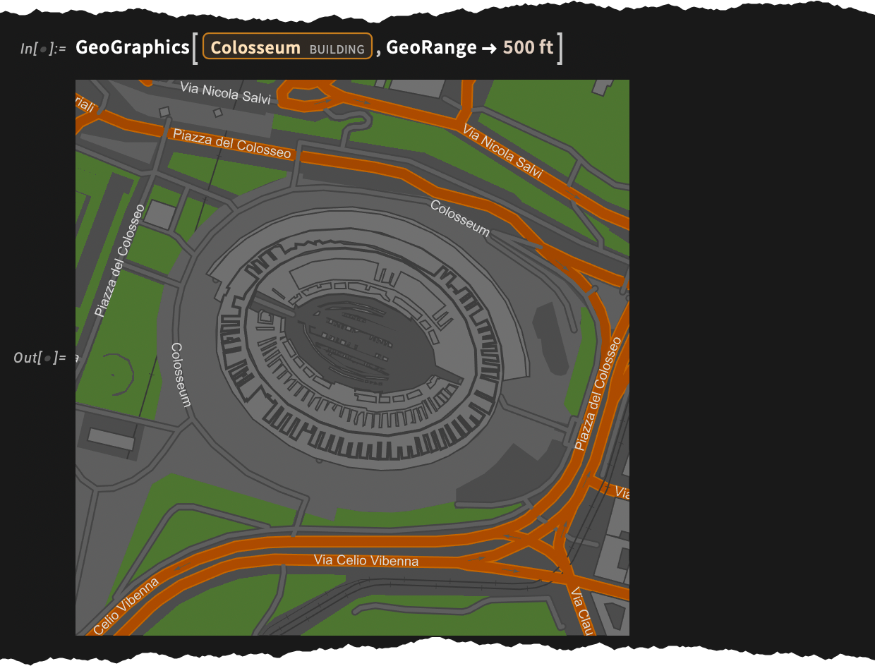
If we look at a smaller area, the “terrain” starts to get faded out:

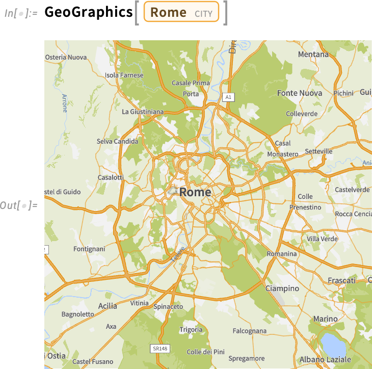
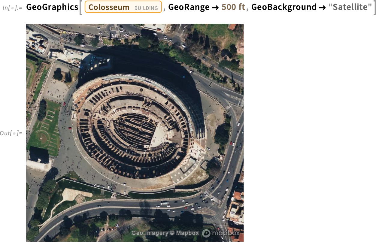
At the level of a city, roads are made prominent (and they’re rendered in new, crisper colors in Version 14.3):

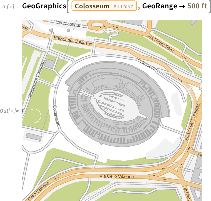
Zooming in further, we see more details:

And, yes, we can get a satellite image too:

Everything has a dark mode:

An important feature of these maps is that they’re all produced with resolution-independent vector graphics. This was a capability we first introduced as an option in Version 12.2, but in Version 14.3 we’ve managed to make it efficient enough that we’ve now set it as the default.

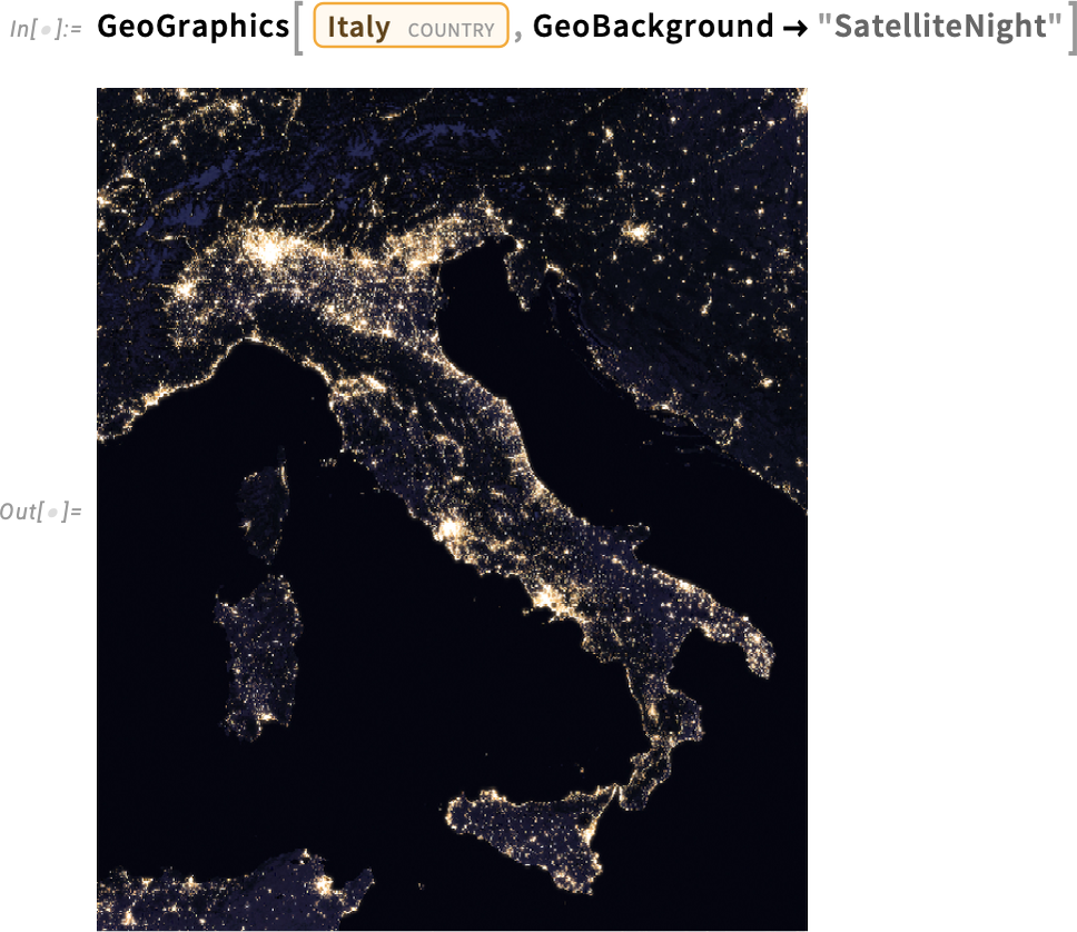
By the way, in Version 14.3 not only can we render maps in dark mode, we can also get actual night-time satellite images:

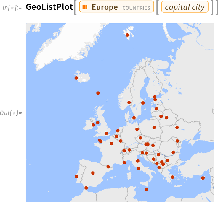
We’ve worked hard to pick nice, crisp colors for our default maps. But sometimes you actually want the “base map” to be quite bland, because what you really want to stand out is data you’re plotting on the map. And so that’s what happens by default in functions like GeoListPlot:

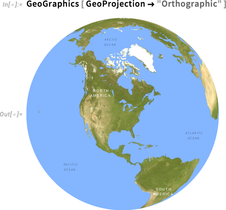
Mapmaking has endless subtleties, some of them mathematically quite complex. Something we finally solved in Version 14.3 is doing true spheroidal geometry on vector geometric data for maps. And a consequence of this is that we can now accurately render (and clip) even very stretched geographic features—like Asia in this projection:

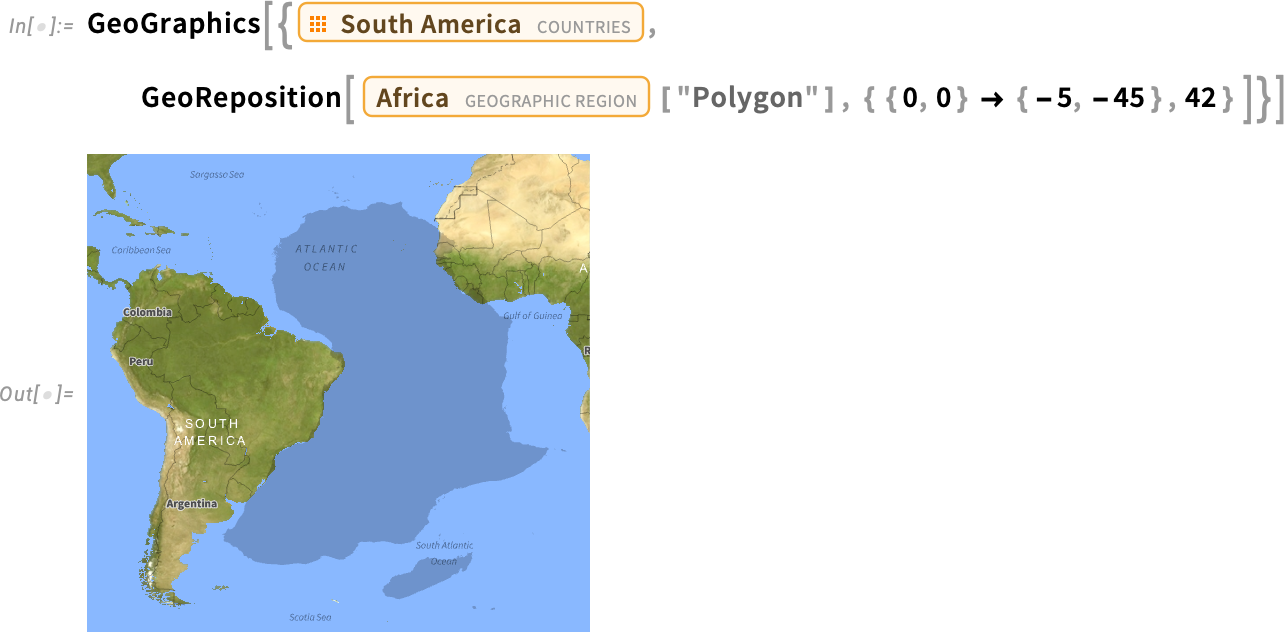
Another new geographic function in Version 14.3 is GeoReposition—which takes a geographic object and transforms its coordinates to move it to a different place on the Earth, preserving its size. So, for example, this shows rather clearly that—with a particular shift and rotation—Africa and South America geometrically fit together (suggesting continental drift):

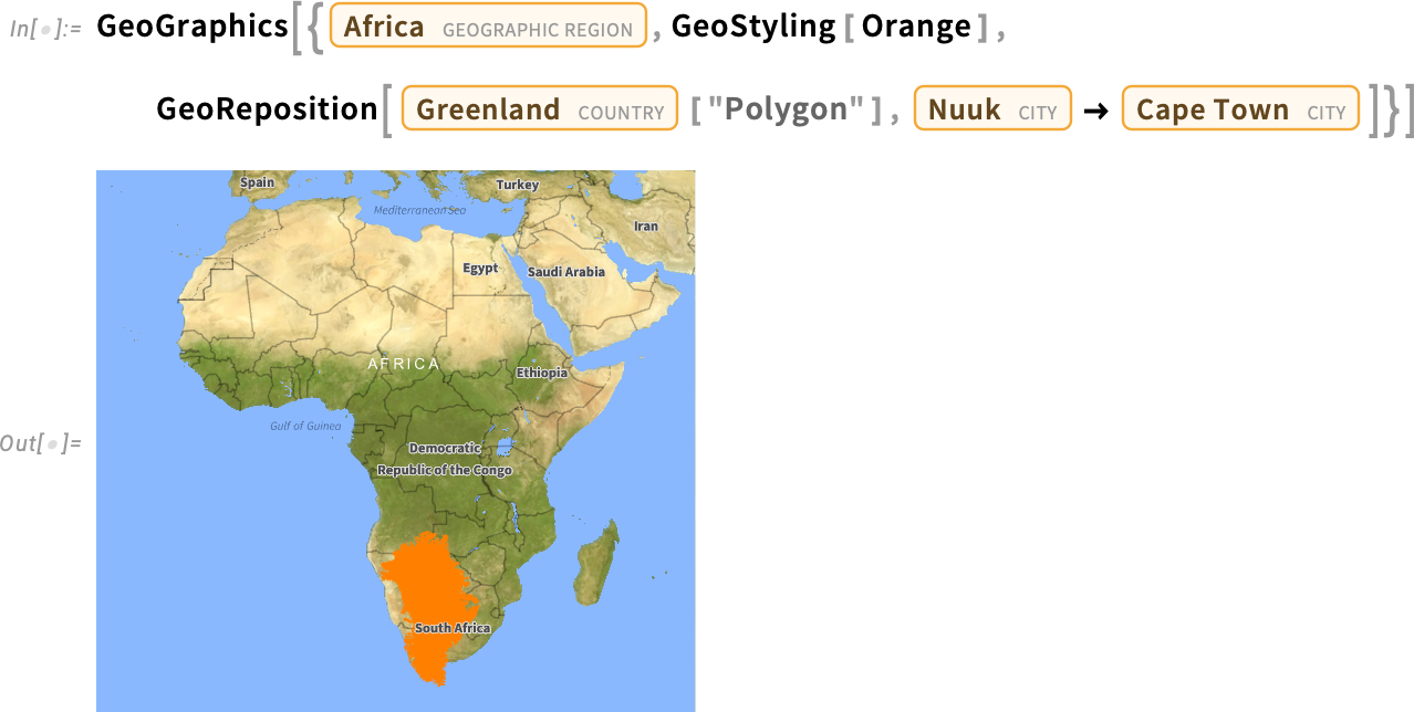
And, yes, despite its appearance on Mercator projection maps, Greenland is not that big:

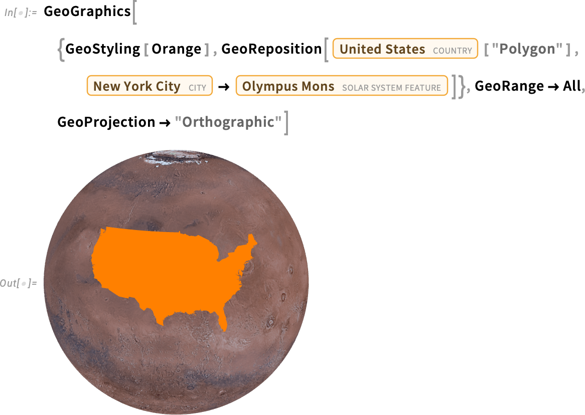
And because in the Wolfram Language we always try to make things as general as possible, yes, you can do this “off planet” as well:

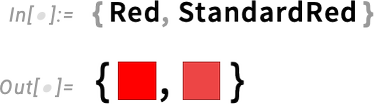
A Better Red: Introducing New Named Colors

“I want to show it in red”, one might say. But what exactly is red? Is it just pure RGBColor[1,0,0], or something slightly different? More than two decades ago we introduced symbols like Red to stand for “pure colors” like RGBColor[1,0,0]. But in making nice-looking, “designed” images, one usually doesn’t want those kinds of “pure colors”. And indeed, a zillion times I’ve found myself wanting to slightly “tweak that red” to make it look better. So in Version 14.3 we’re introducing the new concept of “standard colors”: for example StandardRed is a version of red that “looks red”, but is more “elegant” than “pure red”:

The difference is subtle, but important. For other colors it can be less subtle:

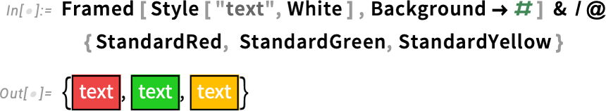
Our new standard colors are picked so that they work well in both light and dark mode:

They also work well not only as foreground colors, but also background colors:

They also are colors that have the same “color weight”, in the sense that—like our default plot colors—they’re balanced in terms of emphasis. Oh, and they’re also selected to go well together.

Here’s an array of all the colors for which we now have symbols (there are White, Black and Transparent as well):

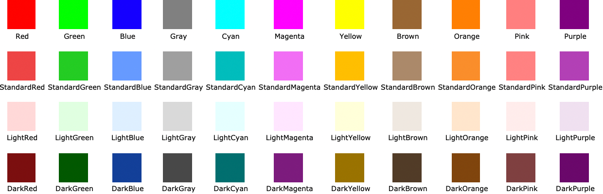
In addition to the “pure colors” and “light colors” which we’ve had for a long time, we’ve not only now added “standard colors”, but also “dark colors”.

So now when you construct graphics, you can immediately get your colors to have a “designer quality” look just by using StandardRed, DarkRed, etc. instead of plain old pure Red.

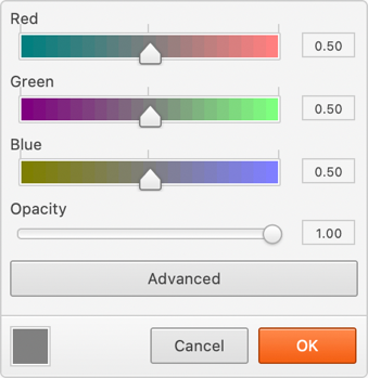
The whole story of dark mode and ligh0t-dark switching introduces yet another issue in the specification of colors. Click any color swatch in a notebook, and you’ll get an interactive color picker:

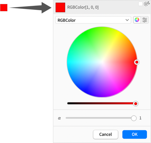
But in Version 14.3 this color picker has been pretty much completely redesigned, both to handle light and dark modes, and generally to streamline the picking of colors.

Previously you’d by default have to pick colors with sliders:

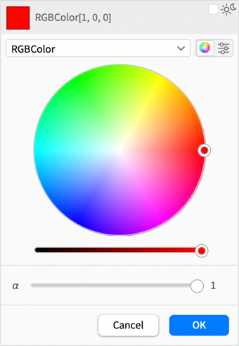
Now there’s a much-easier-to-use color wheel, together with brightness and opacity sliders:

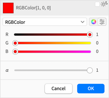
If you want sliders, then you can ask for those too:

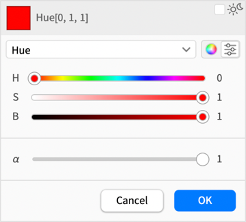
But now you can choose different color spaces—like Hue, which makes the sliders more useful:

What about light-dark switching? Well, the color picker now has this in its right-hand corner:

Click it, and the color you get will be set up to automatically switch in light and dark mode:

Selecting either or you get:

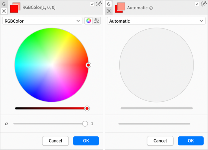
In other words, in this case, the light mode color was explicitly picked, and the dark mode color was generated automatically.

If you really want to have control over everything, you can use the color space menu for dark mode here, and pick not Automatic, but an explicit color space, and then pick a dark mode color manually in that color space.

And, by the way, as another subtlety, if your notebook was in dark mode, things would be reversed, and you’d instead by default be offered the opportunity to pick the dark mode color, and have the light mode color be generated automatically.

More Spiffing Up of Graphics

Version 14.2 had all sorts of great new features. But one “little” enhancement that I see—and appreciate—every day is the “spiffing up” that we did of default colors for plots. Just replacing by , by , by , etc. instantly gave our graphics more “zing”, and generally made them look “spiffier”. So now in Version 14.3 we’ve continued this process, “spiffing up” default colors generated by all sorts of functions.

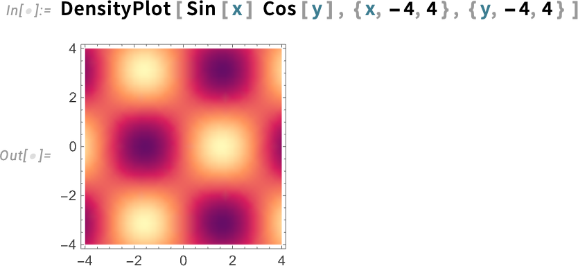
For example, until Version 14.2 the default colors for DensityPlot were

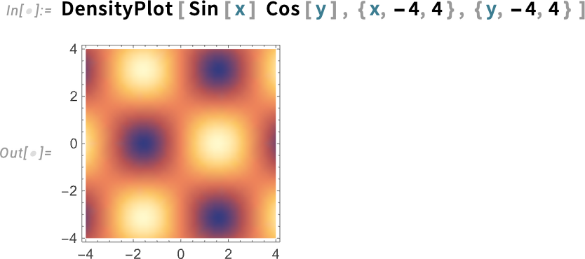
but now “with more zing” they’re:

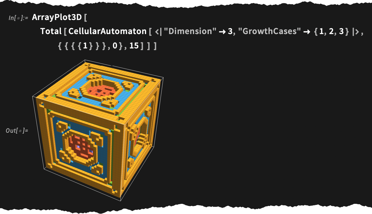
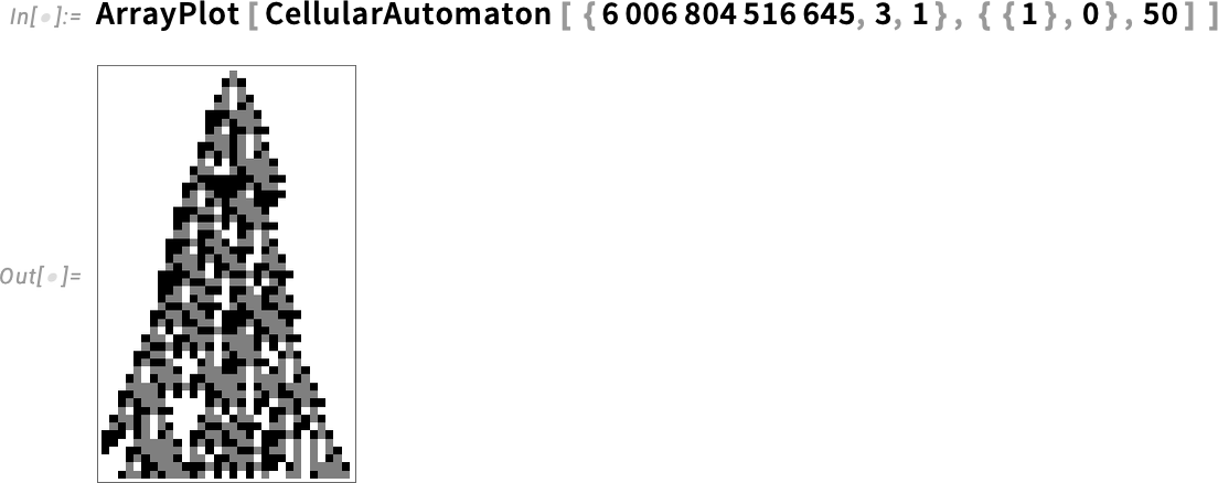
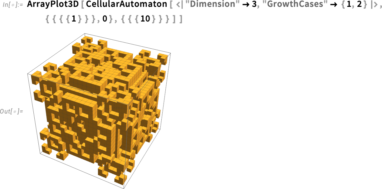
Another example—of particular relevance to me, as a longtime explorer of cellular automata—is an update to ArrayPlot. By default, ArrayPlot uses gray levels for successive values (here just 0, 1, 2):

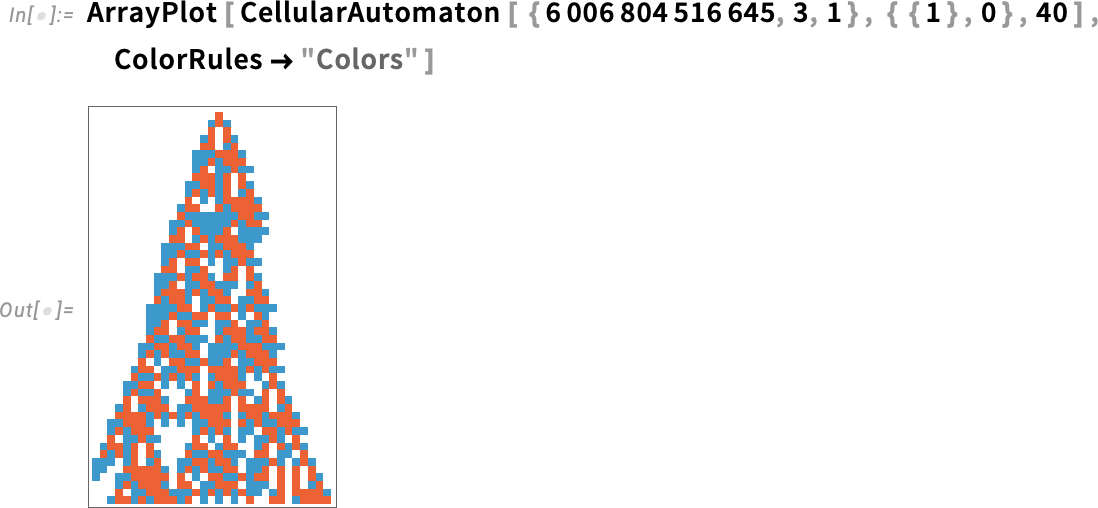
But in Version 14.3, there’s a new option setting—ColorRules"Colors"—that instead uses colors:

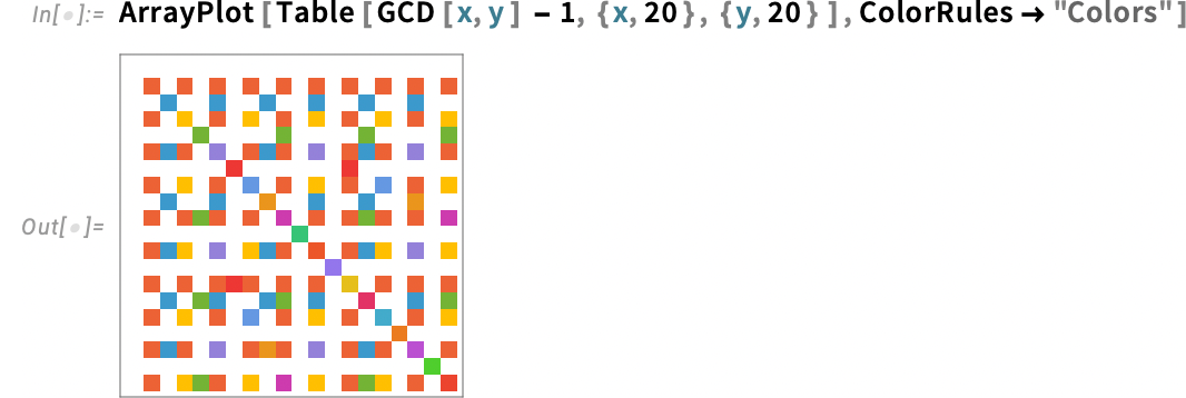
And, yes, it also works for larger numbers of values:

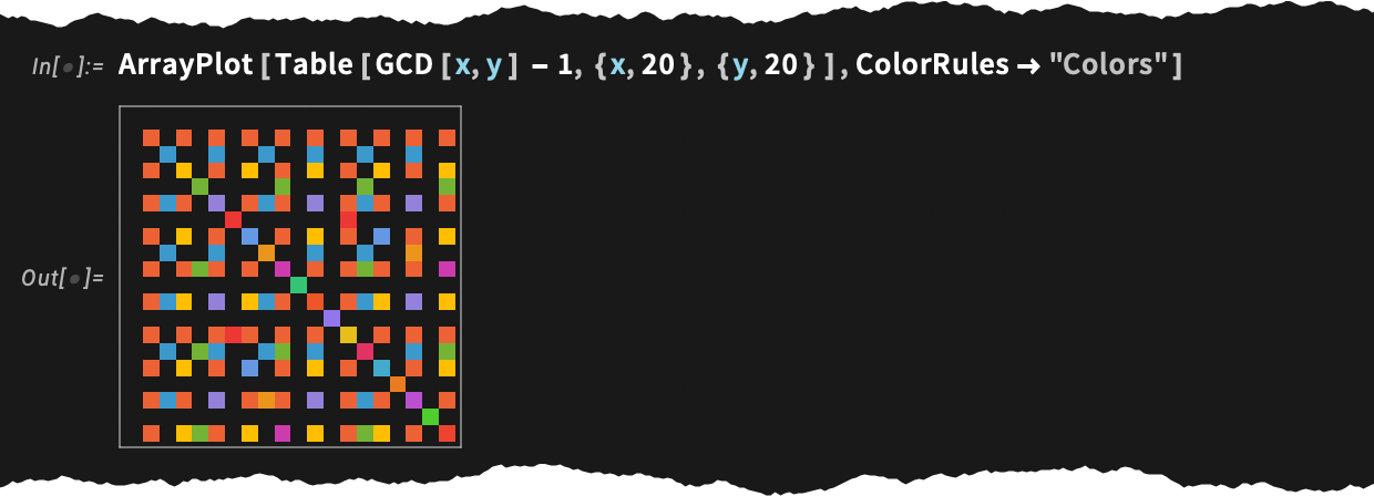
As well as in dark mode:

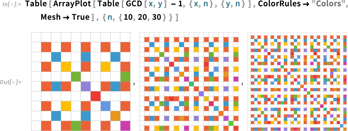
By the way, in Version 14.3 we’ve also improved the handling of meshes—so that they gradually fade out when there are more cells:

What about 3D? We’ve changed the default even with just 0 and 1 to include a bit of color:

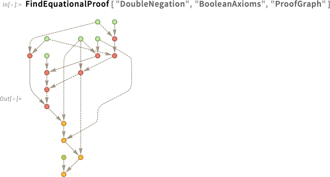
There are updates to colors (and other details of presentation) in many corners of the system. An example is proof objects. In Version 14.2, this was a typical proof object:

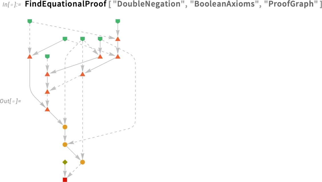
Now in Version 14.3 it looks (we think) a bit more elegant:

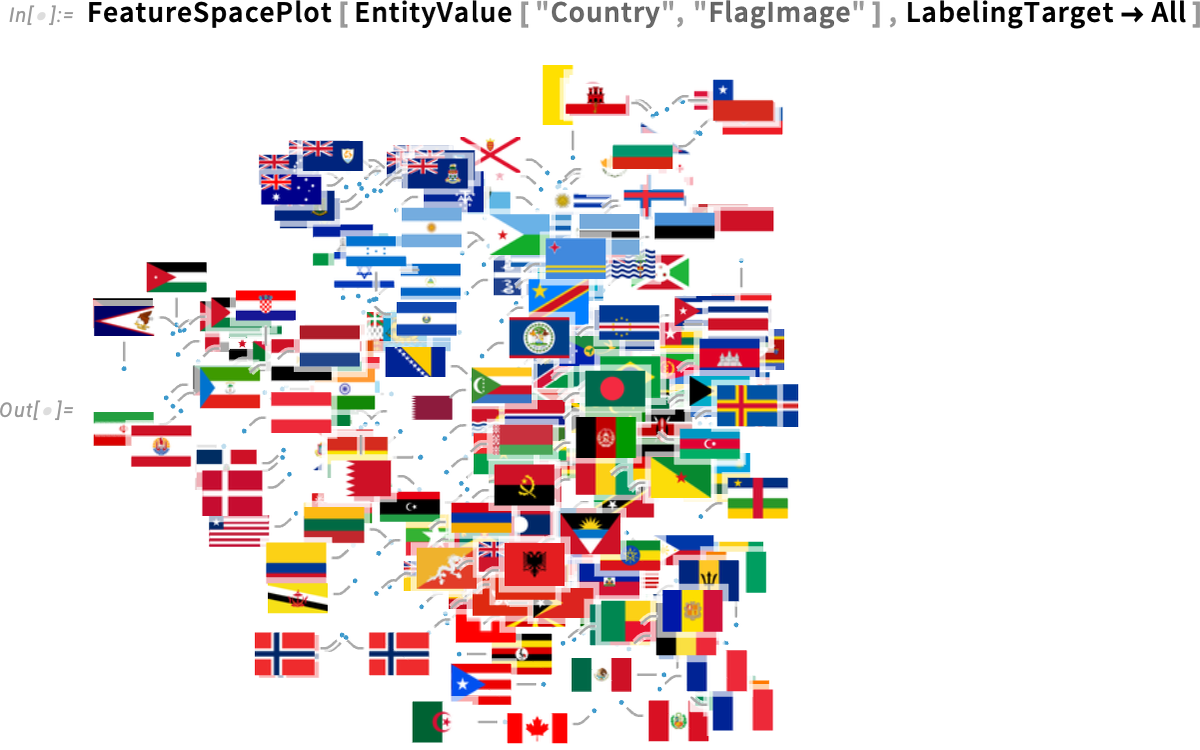
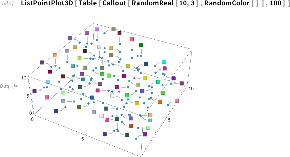
In addition to colors, another significant update in Version 14.3 has to do with labeling in plots. Here’s a feature space plot of images of country flags:

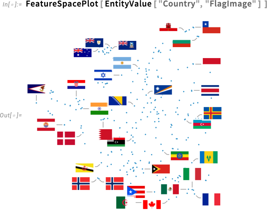
By default, some of the points are labeled, and some are not. The heuristics that are used try to put labels in empty spaces, and when there aren’t enough (or labels would end up overlapping too much), the labels are just omitted. In Version 14.2 the only choice was whether to have labels at all, or not. But now in Version 14.3 there’s a new option LabelingTarget that specifies what to aim for in adding labels.

For example, with LabelingTargetAll, every point is labeled, even if that means there are labels that overlap points, or each other:

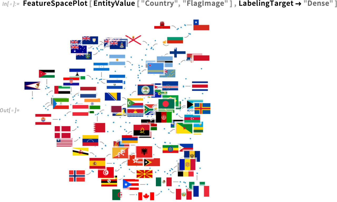
LabelingTarget has a variety of convenient settings. An example is "Dense":

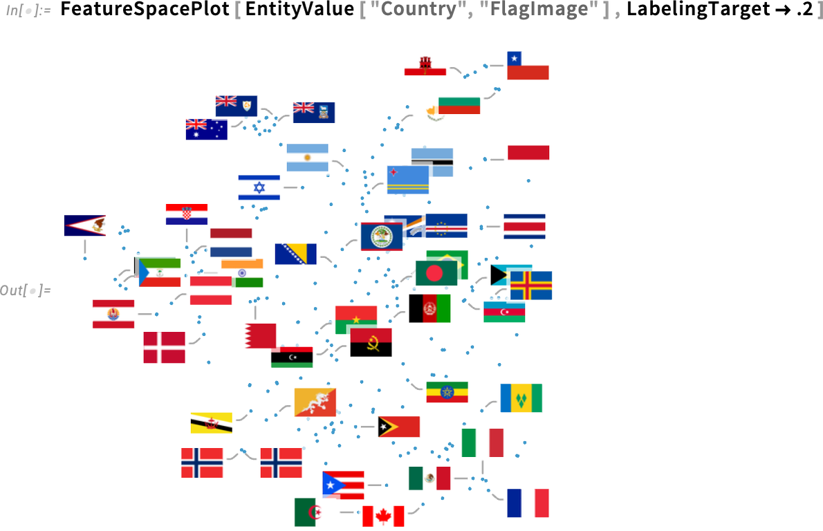
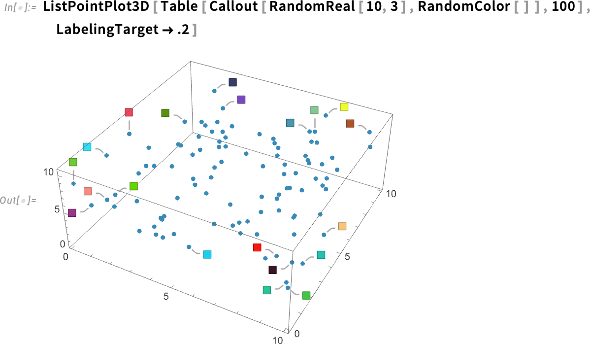
You can also give a number, specifying the fraction of points that should be labeled:

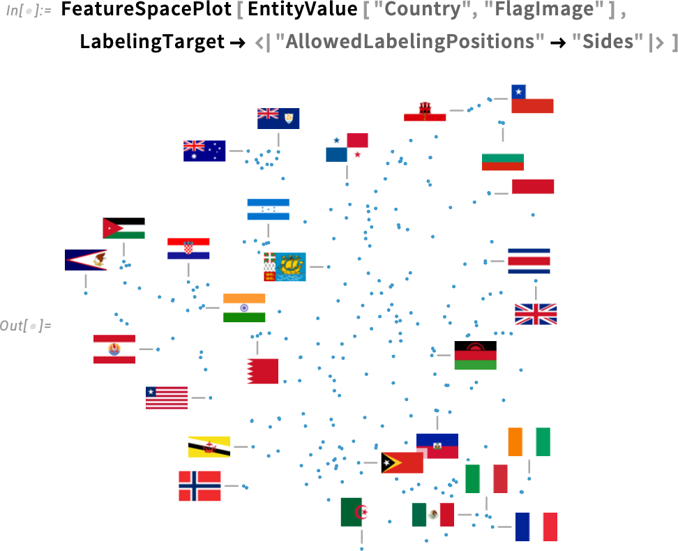
If you want to get into more detail, you can give an association. Like here this specifies that the leaders for all labels should be purely horizontal or vertical, not diagonal:

The option LabelingTarget is supported in the full range of visualization functions that deal with points, both in 2D and 3D. Here’s what happens in this case by default:

And here’s what happens if we ask for “20% coverage”:

In Version 14.3 there are all sorts of new upgrades to our visualization capabilities, but there’s also one (very useful) feature that one can think of as a “downgrade”: the option PlotInteractivity that one can use to switch off interactivity in a given plot. For example, with PlotInteractivityFalse, the bins in a histogram will never “pop” when you mouse over them. And this is useful if you want to ensure efficiency of large and complex graphics, or you’re targeting your graphics for print, etc. where interactivity will never be relevant.

Non-commutative Algebra

“Computer algebra” was one of the key features of Version 1.0 all the way back in 1988. Mainly that meant doing operations with polynomials, rational functions, etc.—though of course our general symbolic language always allowed many generalizations to be made. But all the way back in Version 1.0 we had the symbol NonCommutativeMultiply (typed as **) that was intended to represent a “general non-commutative form of multiplication”. When we introduced it, it was basically just a placeholder, and more than anything else, it was “reserved for future expansion”. Well, 37 years later, in Version 14.3, the algorithms are ready, and the future is here! And now you can finally do computation with NonCommutativeMultiply. And the results can be used not only for “general non-commutative multiplication” but also for things like symbolic array simplification, etc.

Ever since Version 1.0 you’ve been able to enter NonCommutativeMultiply as **. And the first obvious change in Version 14.3 is that now ** automatically turns into ⦻. To support math with ⦻ there’s now also GeneralizedPower which represents repeated non-commutative multiplication, and is displayed as a superscript with a little dot: .

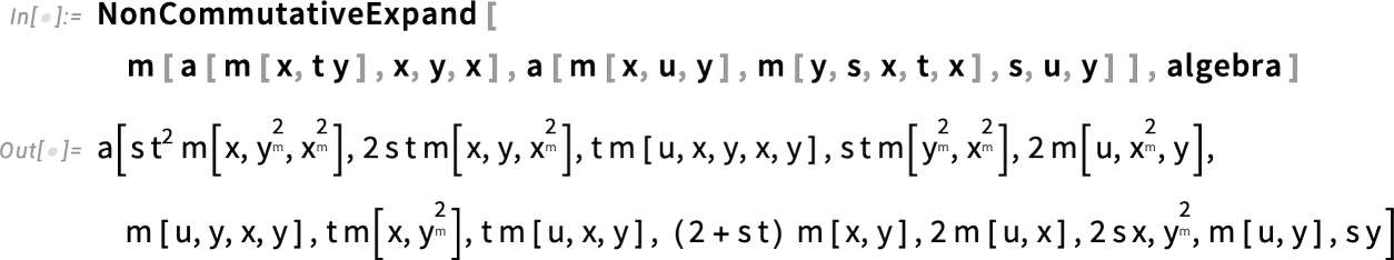
OK, so what about doing operations on expressions containing ⦻? In Version 14.3 there’s NonCommutativeExpand:

By doing this expansion we’re getting a canonical form for our non-commutative polynomial. In this case, FullSimplify can simplify it

though in general there isn’t a unique “factored” form for non-commutative polynomials, and in some (fairly rare) cases the result can be different from what we started with.

⦻ represents a completely general no-additional-relations form of non-commutative multiplication. But there are many other forms of non-commutative multiplication that are useful. A notable example is . (Dot). In Version 14.2 we introduced ArrayExpand which operates on symbolic arrays:

Now we have NonCommutativeExpand, which can be told to use Dot as its multiplication operation:

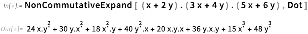
The result looks different, because it’s using GeneralizedPower. But we can use FullSimplify to check the equivalence:

The algorithms we’ve introduced around non-commutative multiplication now allow us to do more powerful symbolic array operations, like this piece of array simplification:

How does it work? Well, at least in multivariate situations, it’s using the non-commutative version of Gröbner bases. Gröbner bases are a core method in ordinary, commutative polynomial computation; in Version 14.3 we’ve generalized them to the non-commutative case:

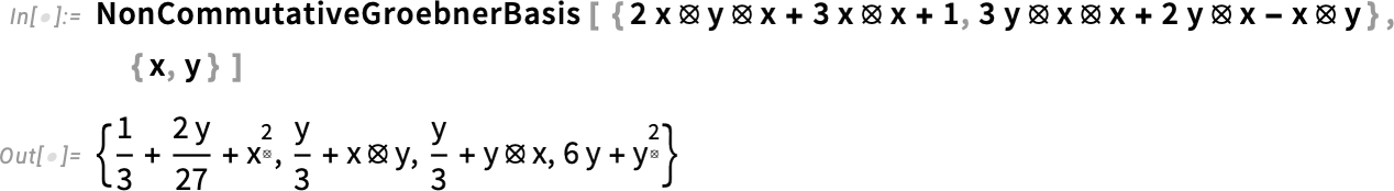
To get a sense of what kind of thing is going on here, let’s look at a simpler case:

We can think of the input as giving a list of expressions that are assumed to be zero. And by including, for example, a⦻b–1 we’re effectively asserting that a⦻b=1, or, put another way, that b is a right inverse of a. So in effect we’re saying here that b is a right inverse of a, and c is a left inverse. The Gröbner basis that’s output then also includes b–c, showing that the conditions we’ve specified imply that b–c is zero, i.e. that b is equal to c.

Non-commutative algebras show up all over the place, not only in math but also in physics (and particularly quantum physics). They can also be used to represent a symbolic form of functional programming. Like here we’re collecting terms with respect to f, with the multiplication operation being function composition:

In many applications of non-commutative algebra, it’s useful to have the notion of a commutator:

And, yes, we can check famous commutation relations, like ones from physics:

(There’s AntiCommutator as well.)

A function like NonCommutativeExpand by default assumes that you’re dealing with a non-commutative algebra in which addition is represented by + (Plus), multiplication by ⦻ (NonCommutativeMultiply), and that 0 is the identity for +, and 1 for ⦻. But by giving a second argument, you can tell NonCommutativeExpand that you want to use a different non-commutative algebra. {Dot, n}, for example, represents an algebra of n×n matrices, where the multiplication operation is . (Dot), and the identity, for example, is n (SymbolicIdentityArray[n]). TensorProduct represents an algebra of formal tensors, with  (TensorProduct) as its multiplication operation. But in general you can define your own non-commutative algebra with NonCommutativeAlgebra:

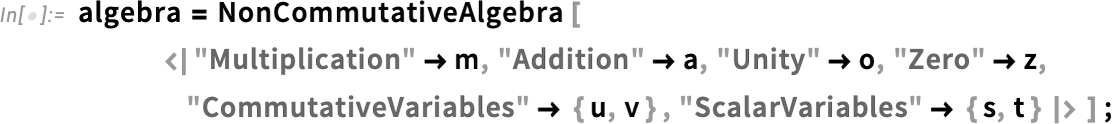
Now we can expand an expression assuming it’s an element of this algebra (note the tiny m’s in the generalized “m powers”):

Draw on That Surface: The Visual Annotation of Regions

You’ve got a function of x, y, z, and you’ve got a surface embedded in 3D. But how do you plot that function over the surface? Well, in Version 14.3 there’s a function for that:

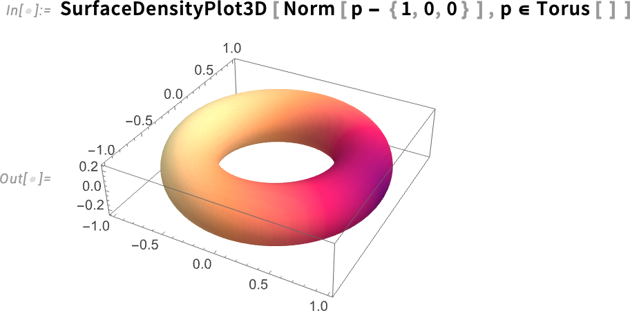
You can do this over the surface of any kind of region:

There’s a contour plot version as well:

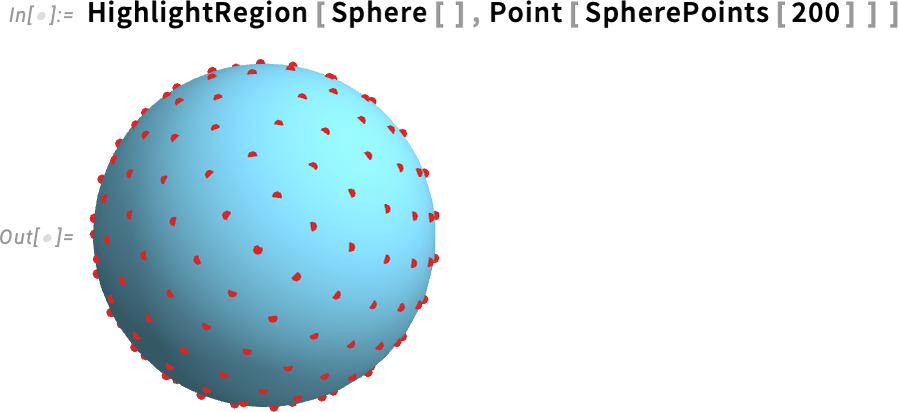
But what if you don’t want to plot a whole function over a surface, but you just want to highlight some particular aspect of the surface? Then you can use the new function HighlightRegion. You give HighlightRegion your original region, and the region you want to highlight on it. So, for example, this highlights 200 points on the surface of a sphere (and, yes, HighlightRegion correctly makes sure you can see the points, and they don’t get “sliced” by the surface):

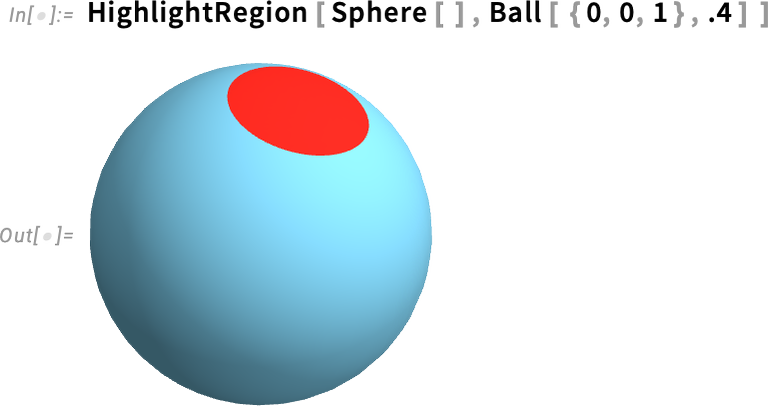
Here we’re highlighting a cap on a sphere (specified as the intersection between a ball and the surface of the sphere):

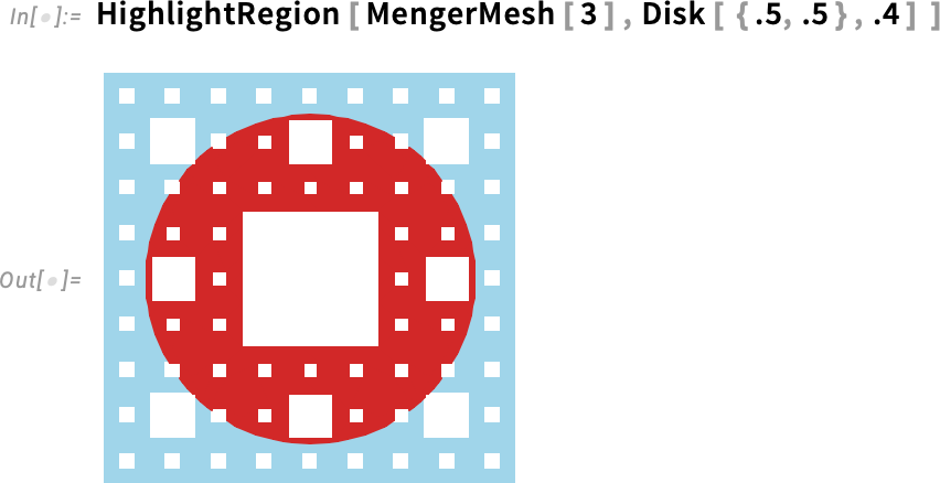
HighlightRegion works not just in 3D but for regions in any number of dimensions:

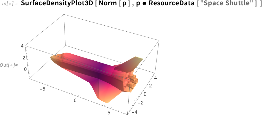
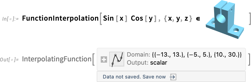
Coming back to functions on surfaces, another convenient new feature of Version 14.3 is that FunctionInterpolation can now work over arbitrary regions. The goal of FunctionInterpolation is to take some function (which might be slow to compute) and to generate from it an InterpolatingFunction object that approximates the function. Here’s an example where we’re now interpolating a fairly simple function over a complicated region:

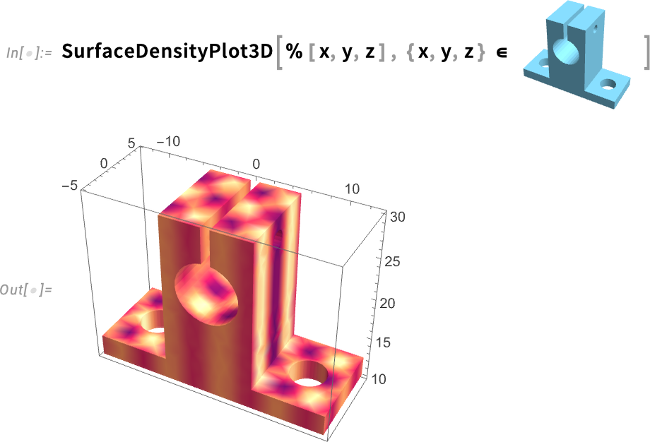
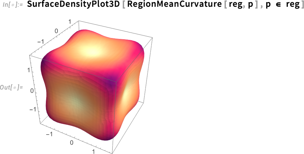
Now we can use SurfaceDensityPlot3D to plot the interpolated function over the surface:

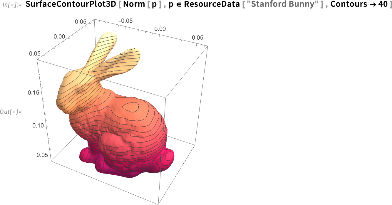
Curvature Computation & Visualization

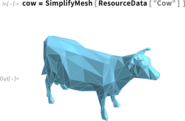
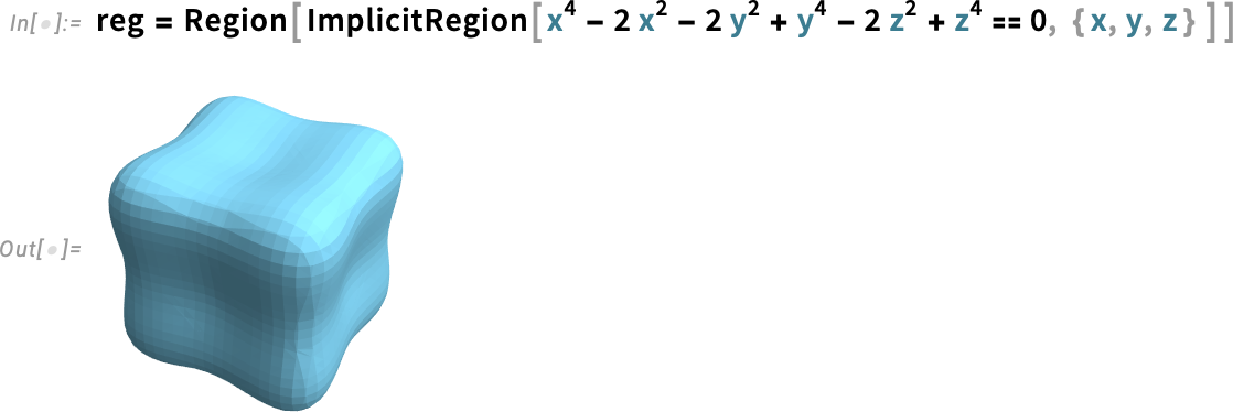
Let’s say we’ve got a 3D object:

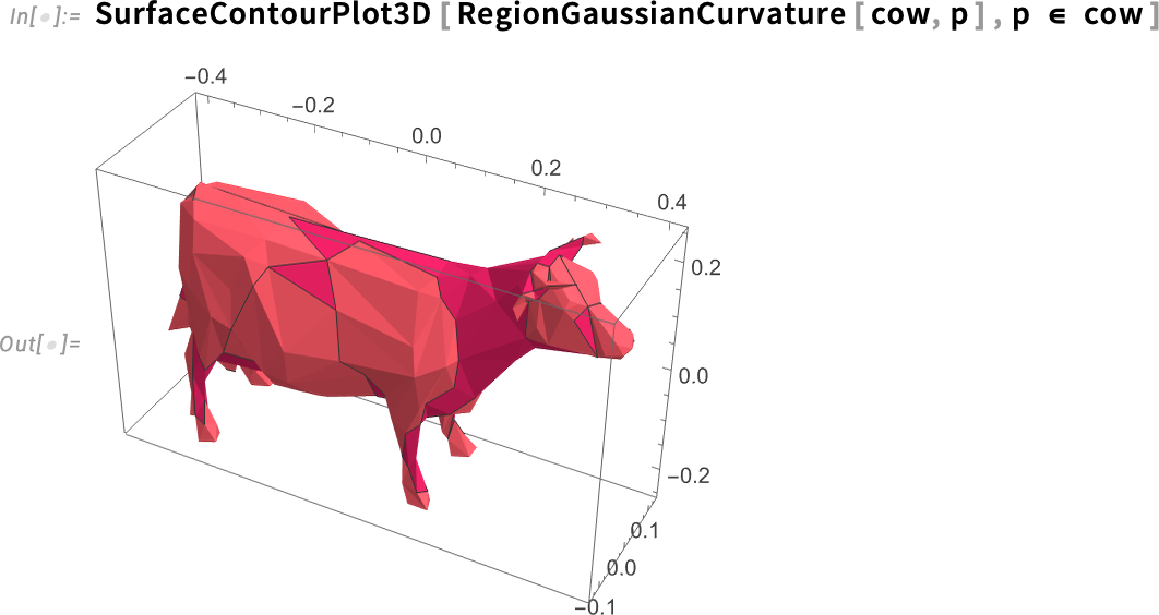
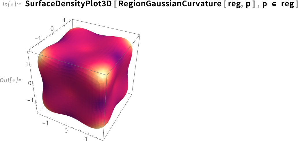
In Version 14.3 we can now compute the Gaussian curvature of its surface. Here we’re using the function SurfaceContourPlot3D to plot a value on a surface, with the variable p ranging over the surface:

In this example, our 3D object is specified purely by a mesh. But let’s say we have a parametric object:

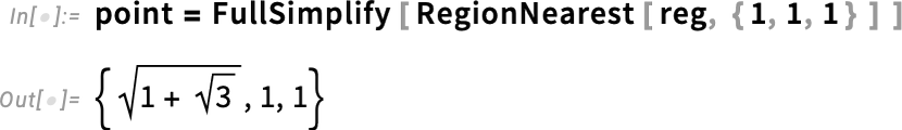
Again we can compute the Gaussian curvature:

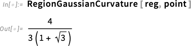
But now we can get exact results. Like this finds a point on the surface:

And this then computes the exact value of the Gaussian curvature at that point:

Version 14.3 also introduces mean curvature measures for surfaces

as well as max and min curvatures:

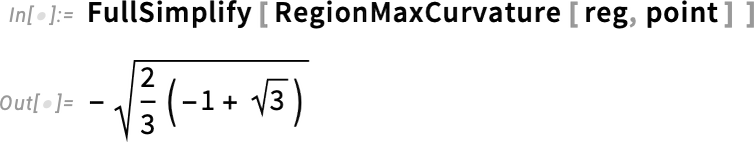
These surface curvatures are in effect 3D generalizations of the ArcCurvature that we introduced more than a decade ago (in Version 10.0): the min and max curvatures correspond to the min and max curvatures of curves laid on the surface; the Gaussian curvature is the product of these, and the mean curvature is their mean.

Geodesics & Path Planning

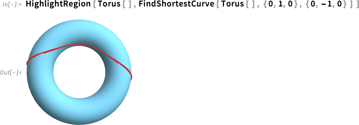
What’s the shortest path from one point to another—say on a surface? In Version 14.3 you can use FindShortestCurve to find out. As an example, let’s find the shortest path (i.e. geodesic) between two points on a sphere:

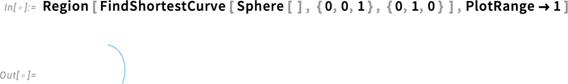
Yes, we can see a little arc of what seems like a great circle. But we’d really like to visualize it on the sphere. Well, we can do that with HighlightRegion:

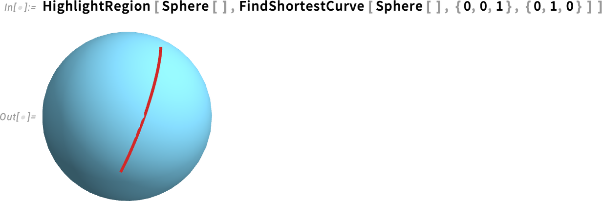
Here’s a similar result for a torus:

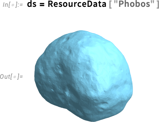
But, actually, any region whatsoever will work. Like, for example, Phobos, a moon of Mars:

Let’s pick two random points on this:

Now we can find the shortest curve between these points on the surface:

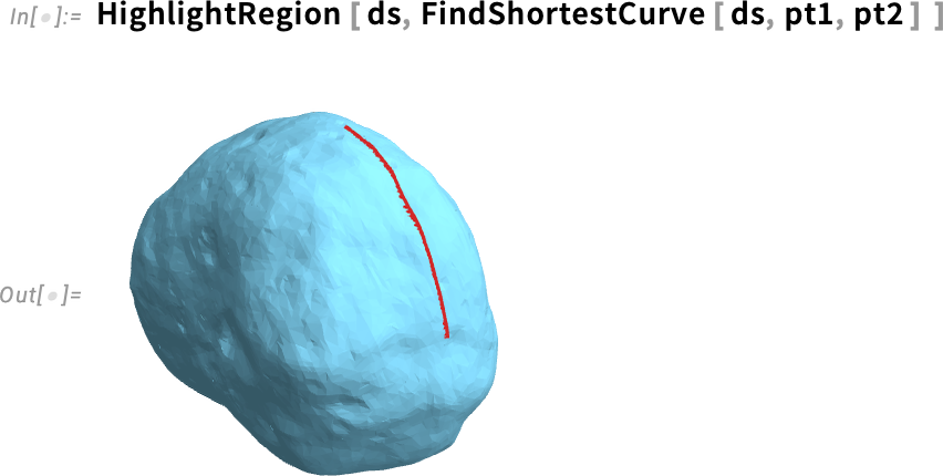
You could use ArcLength to find the length of this curve, or you can directly use the new function ShortestCurveDistance:

Here are 25 geodesics between random pairs of points:

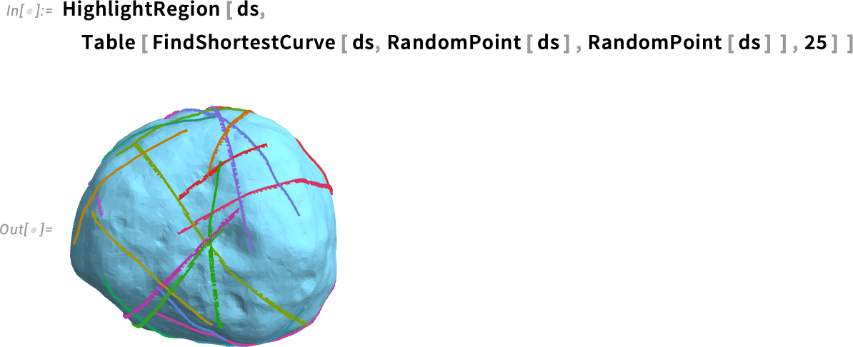
And, yes, the region can be complicated; FindShortestCurve can handle it. But the reason it’s a “Find…” function is that in general there can be many paths of the same length:

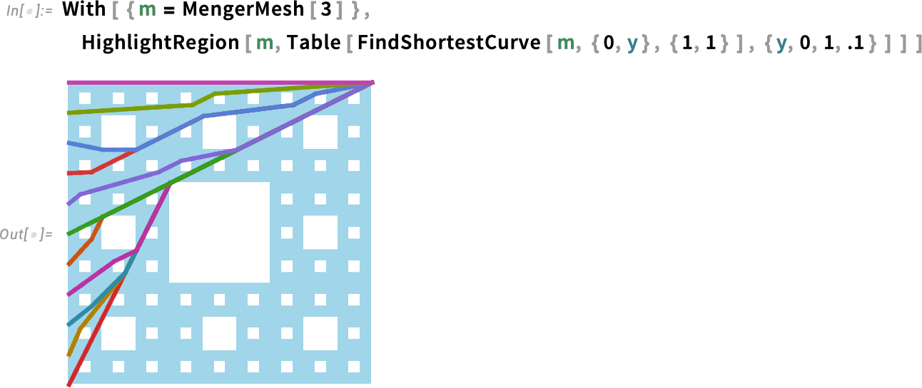
We’ve been looking so far at surfaces in 3D. But FindShortestCurve
also works in 2D:

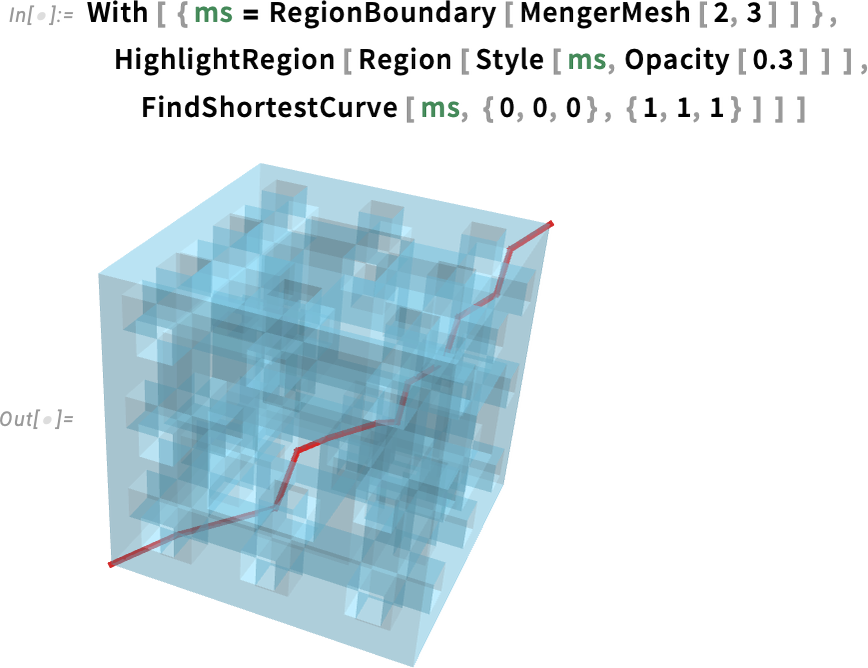
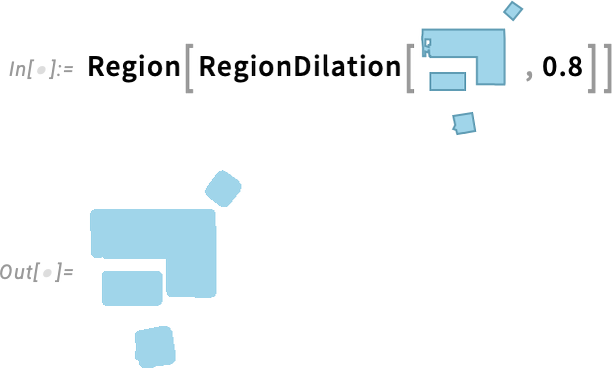
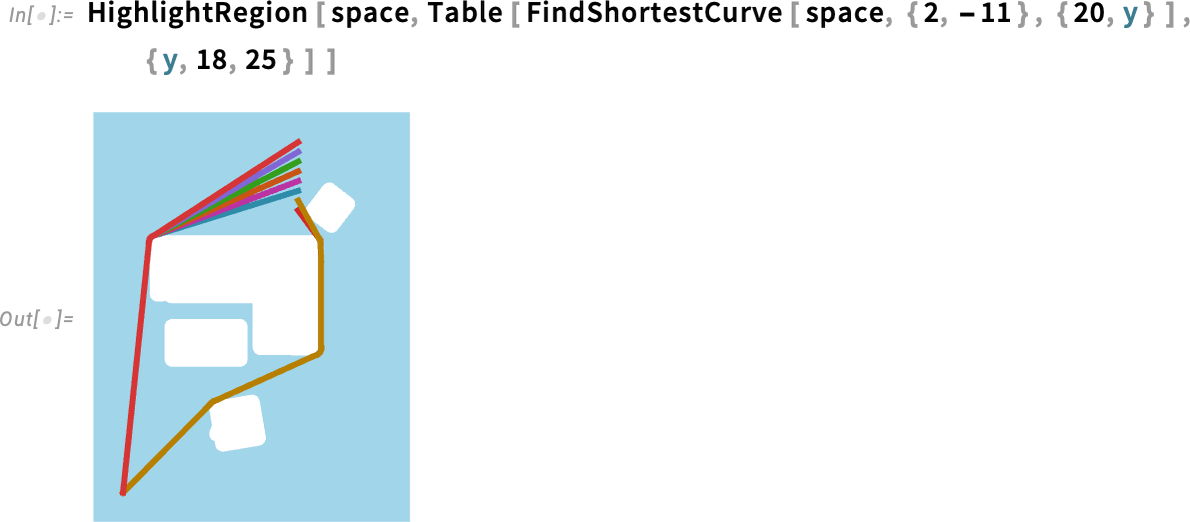
So what is this good for? Well, one thing is path planning. Let’s say we’re trying to make a robot get from here to there, avoid obstacles, etc. What is the shortest path it can take? That’s something we can use FindShortestCurve for. And if we want to deal with the “size of the robot” we can do that by “dilating our obstacles”. So, for example, here’s a plan for some furniture:

Let’s now “dilate” this to give the effective region for a robot of radius 0.8:

Inverting this relative to a “rug” now gives us the effective region that the (center of the) robot can move in:

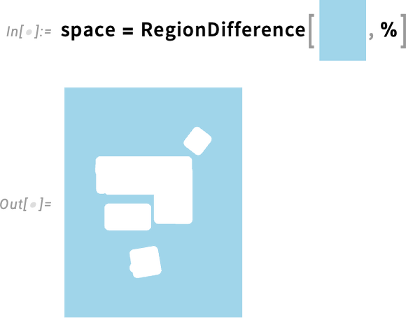
Now we can use FindShortestCurve to find the shortest paths for the robot to get to different places:

Geometry from Subdivision

Creating “realistic” geometry is hard, particularly in 3D. One way to make it easier is to construct what you want by combining basic shapes (say spheres, cylinders, etc.). And we’ve supported that kind of “constructive geometry” since Version 13.0. But now in Version 14.3, there’s another, powerful alternative: starting with a skeleton of what you want, and then filling it in by taking the limit of an infinite number of subdivisions. So, for example, we might start from a very coarse, faceted approximation to the geometry of a cow, and by doing subdivisions we fill it in to a smooth shape:

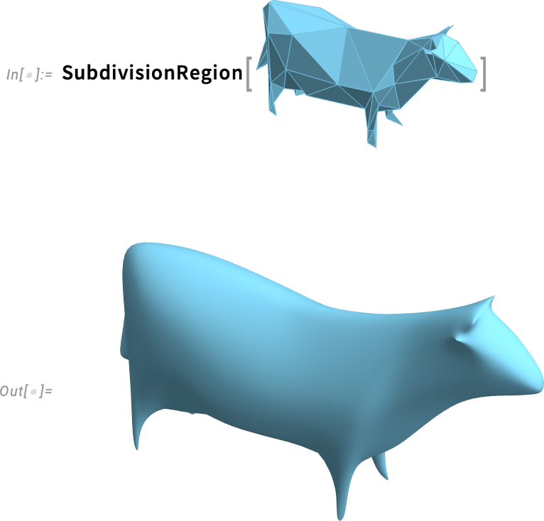
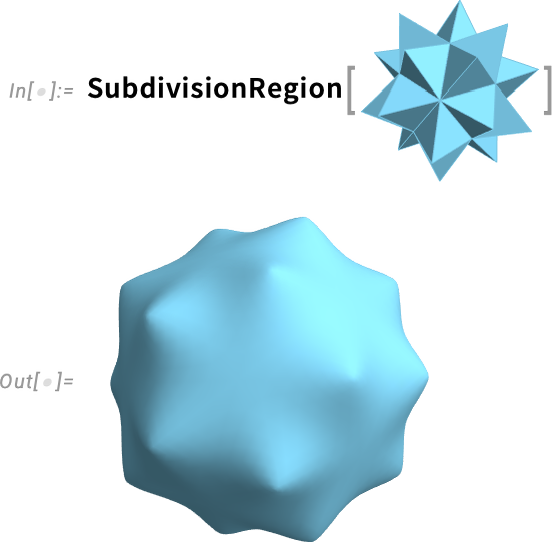
It’s pretty typical to start from something “mathematical looking”, and end with something more “natural” or “biological”:

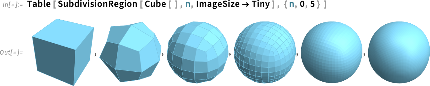
Here’s what happens if we start from a cube, and then do successive steps of subdividing each face:

As a more realistic example, say we start with an approximate mesh for a bone:

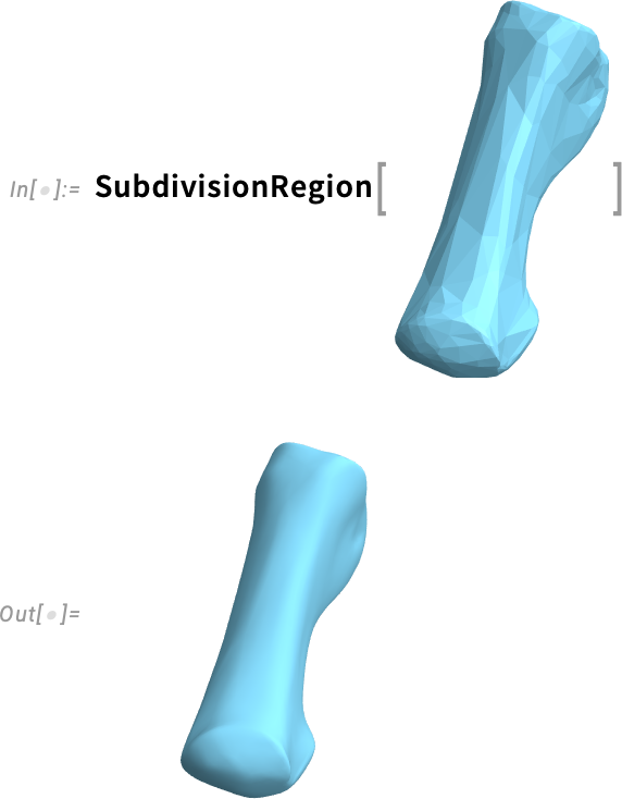
SubdivisionRegion immediately gives a us a smoothed—and presumably more realistic—version.

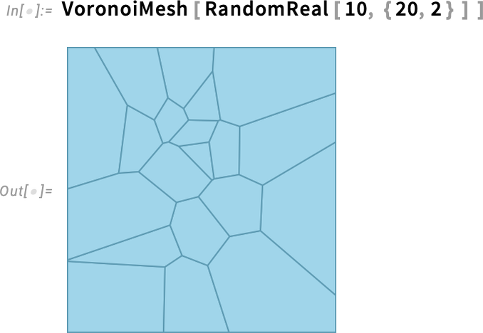
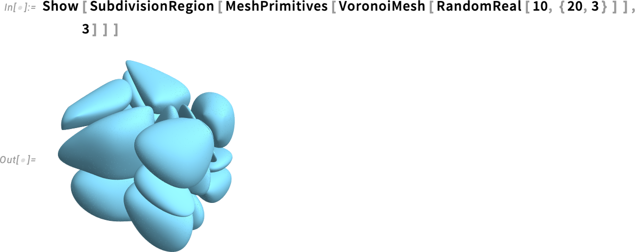
Like other computational geometry in the Wolfram Language, SubdivisionRegion works not only in 3D, but also in 2D. So, for example, we can take a random Voronoi mesh

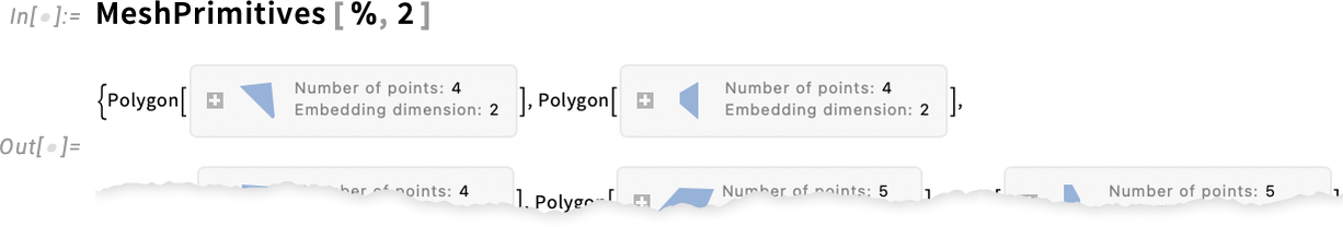
then split it into polygonal cells

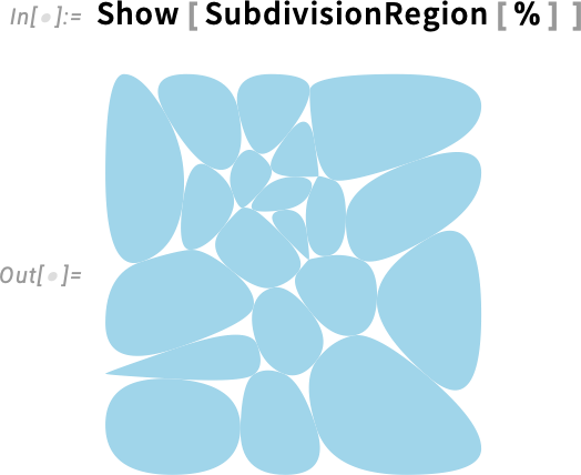
and then make subdivision regions from these to produce a rather “pebble look”:

Or in 3D:

Fix That Mesh!

Let’s say we have a cloud of 3D points, perhaps from a scanner:

The function ReconstructionMesh introduced in Version 13.1 will attempt to reconstruct a surface from this:

It’s pretty common to see this kind of noisy “crinkling”. But now, in Version 14.3, we have a new function that can smooth this out:

That looks nice. But it has a lot of polygons in it. And for some kinds of computations you’ll want a simpler mesh, with fewer polygons. The new function SimplifyMesh can take any mesh and produce an approximation with fewer polygons:

And, yes, it looks a bit more faceted, but the number of polygons is 10x lower:

By the way, another new function in Version 14.3 is Remesh. When you do operations on meshes it’s fairly common to generate “weird” (e.g. very pointy) polygons in the mesh. Such polygons can cause trouble if you’re, say, doing 3D printing or finite element analysis. Remesh creates a new “remeshed” mesh in which weird polygons are avoided.

Color That Molecule—and More

Chemical computation in the Wolfram Language began in earnest six years ago—in Version 12.0—with the introduction of Molecule and many functions around it. And in the years since then we’ve been energetically rounding out the chemistry functionality of the language.

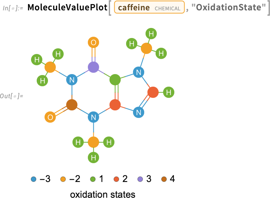
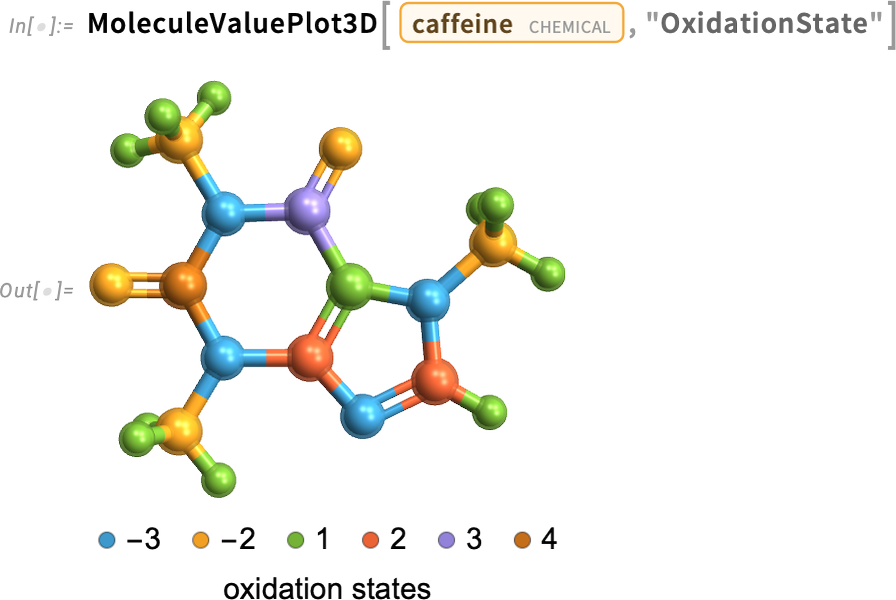
A new capability in Version 14.3 is molecular visualization in which atoms—or bonds—can be colored to show values of a property. So, for example, here are oxidation states of atoms in a caffeine molecule:

And here’s a 3D version:

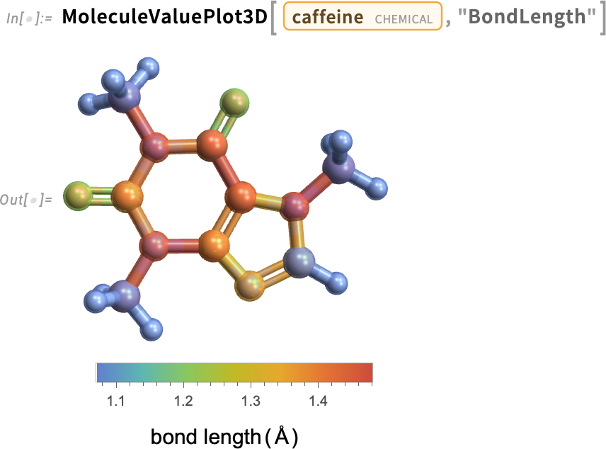
And here’s a case where the quantity we’re using for coloring has a continuous range of values:

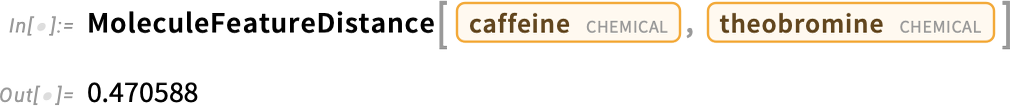
Another new chemistry function in Version 14.3 is MoleculeFeatureDistance—which gives a quantitative way to measure “how similar” two molecules are:

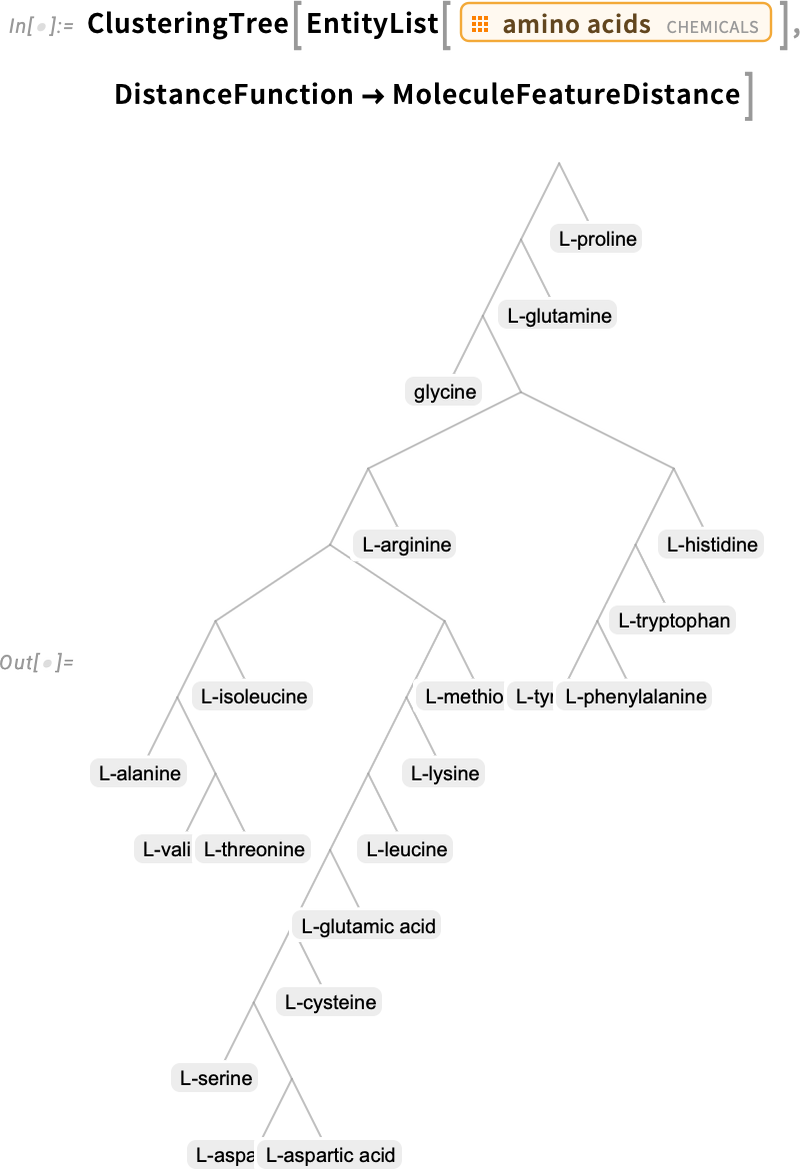
You can use this distance in, for example, making a clustering tree of molecules, here of amino acids:

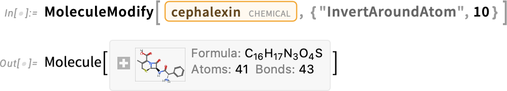
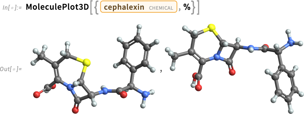
When we first introduced Molecule we also introduced MoleculeModify. And over the years, we’ve been steadily adding more functionality to MoleculeModify. In Version 14.3 we added the ability to invert a molecular structure around an atom, in effect flipping the local stereochemistry of the molecule:

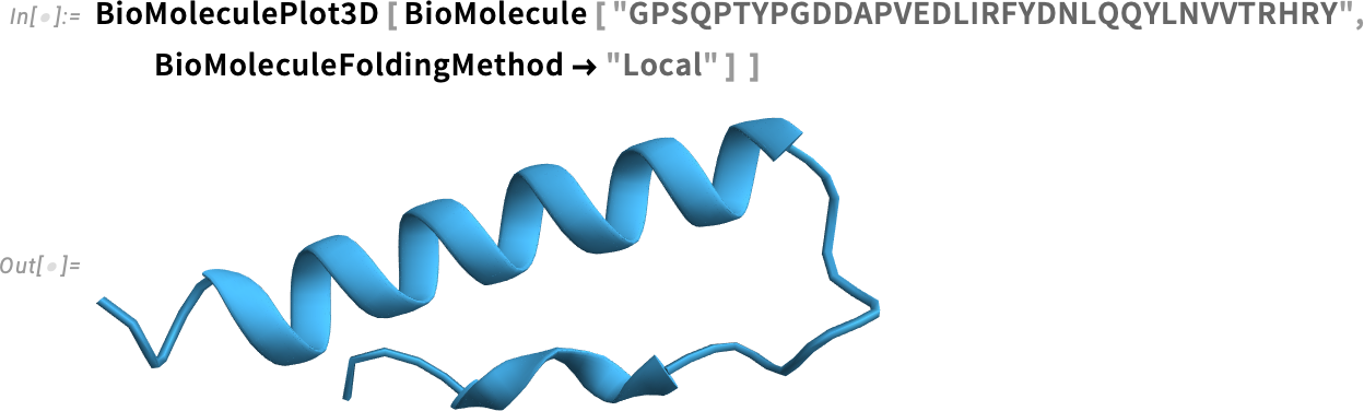
The Proteins Get Folded—Locally

What shape will that protein be? The Wolfram Language has access to a large database of proteins whose structures have been experimentally measured. But what if you’re dealing with a new, different amino acid sequence? How will it fold? Since Version 14.1 BioMolecule has automatically attempted to determine that, but it’s had to call an external API to do so. Now in Version 14.3 we’ve set it up so that you can do the folding locally, on your own computer. The neural net that’s needed is not small—it’s about 11 gigabytes to download, and 30 gigabytes uncompressed on your computer. But being able to work purely locally allows you to systematically do protein folding without the volume and rate limits of an external API.

Here’s an example, doing local folding:

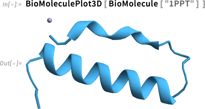
And, remember, this is just a machine-learning-based estimate of the structure. Here’s the experimentally measured structure in this case—qualitatively similar, but not precisely the same:

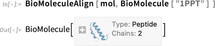
So how can we actually compare these structures? Well, in Version 14.3 there’s a new function BioMoleculeAlign (analogous to MoleculeAlign) that tries to align one biomolecule to another. Here’s our predicted folding again:

Now we align the experimental structure to this:

This now shows the structures together:

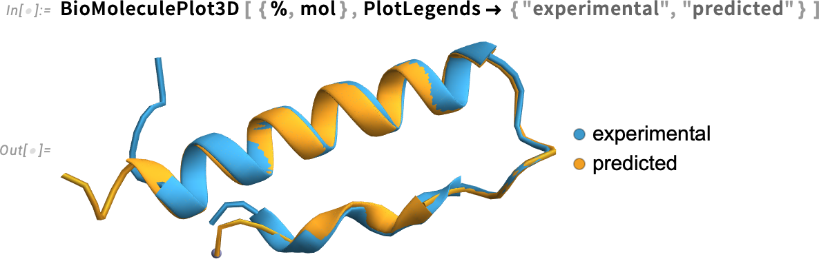
And, yes, at least in this case, the agreement is quite good, and, for example, the error (averaged over core carbon atoms in the backbone) is small:

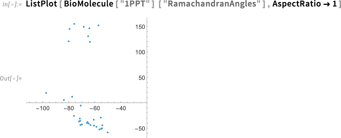
Version 14.3 also introduces some new quantitative measures of “protein shape”. First, there are Ramachandran angles, which measure the “twisting” of the backbone of the protein (and, yes, those two separated regions correspond to the distinct regions one can see in the protein):

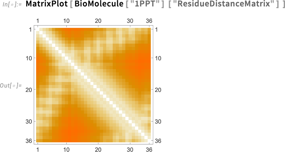
And then there’s the distance matrix between all the residues (i.e. amino acids) in the protein:

Will That Engineering System Actually Work?

For more than a decade Wolfram System Modeler has let one build up and simulate models of real-world engineering and other systems. And by “real world” I mean an expanding range of actual cars, planes, power plants, etc.—with tens of thousands of components—that companies have built (not to mention biomedical systems, etc.) The typical workflow is to interactively construct systems in System Modeler, then to use Wolfram Language to do analysis, algorithmic design, etc. on them. And now, in Version 14.3, we’ve added a major new capability: also being able to validate systems in Wolfram Language.

Will that system stay within the limits that were specified for it? For safety, performance and other reasons, that’s often an important question to ask. And now it’s one you can ask SystemModelValidate to answer. But how do you specify the specifications? Well, that needs some new functions. Like SystemModelAlways—that lets you give a condition that you want the system always to satisfy. Or SystemModelEventually—that lets you give a condition that you want the system eventually to satisfy.

Lets starts with a toy example. Consider this differential equation:

Solve this differential equation and we get:

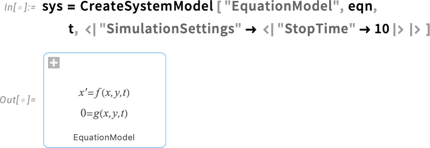
We can set this up as a System Modeler–style model:

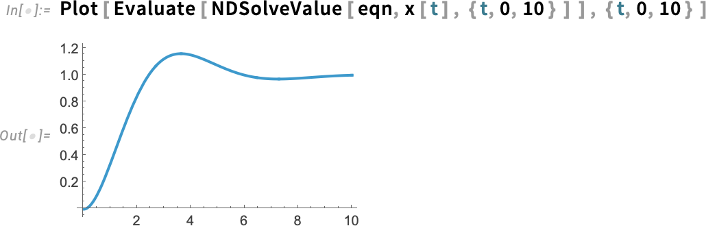
This simulates the system and plots what it does:

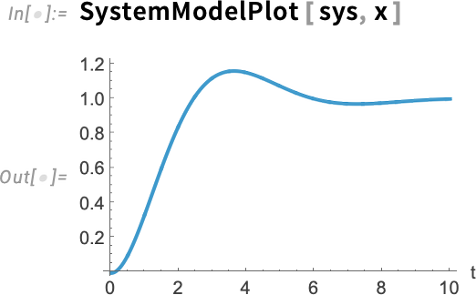
Now let’s say we want to validate the behavior of the system, for example checking whether it ever overshoots value 1.1. Then we just have to say:

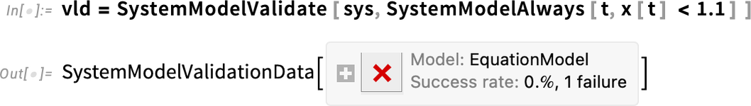
And, yes, as the plot shows, the system doesn’t always satisfy this constraint. Here’s where it fails:

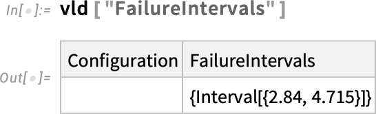
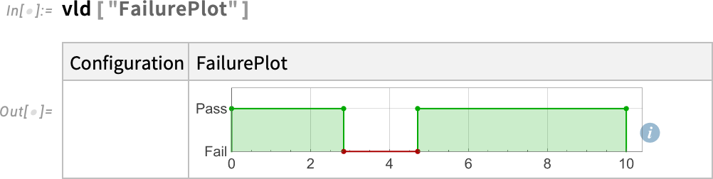
And here’s a visual representation of the region of failure:

OK, well what about a more realistic example? Here’s a slightly simplified model of the drive train of an electric car (with 469 system variables):

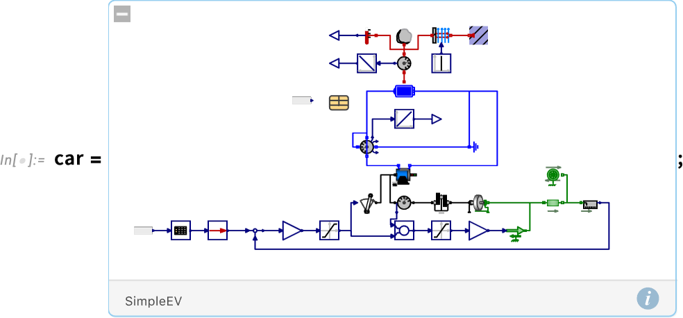
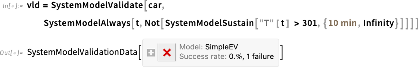
Let’s say we have the specification: “Following the US EPA Highway Fuel Economy Driving Schedule (HWFET) the temperature in the car battery can only be above 301K for at most 10 minutes”. In setting up the model, we already inserted the HWFET “input data”. Now we have to translate the rest of this specification into symbolic form. And for that we need a temporal logic construct, also new in Version 14.3: SystemModelSustain. We end up saying: “check whether it’s always true that the temperature is not sustained as being above 301 for 10 minutes or more”. And now we can run SystemModelValidate and find out if that’s true for our model:

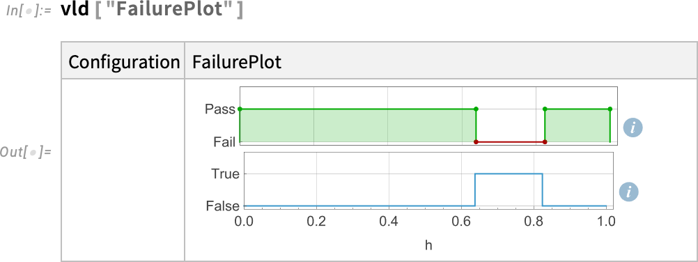
And no, it’s not. But where does it fail? We can make a plot of that:

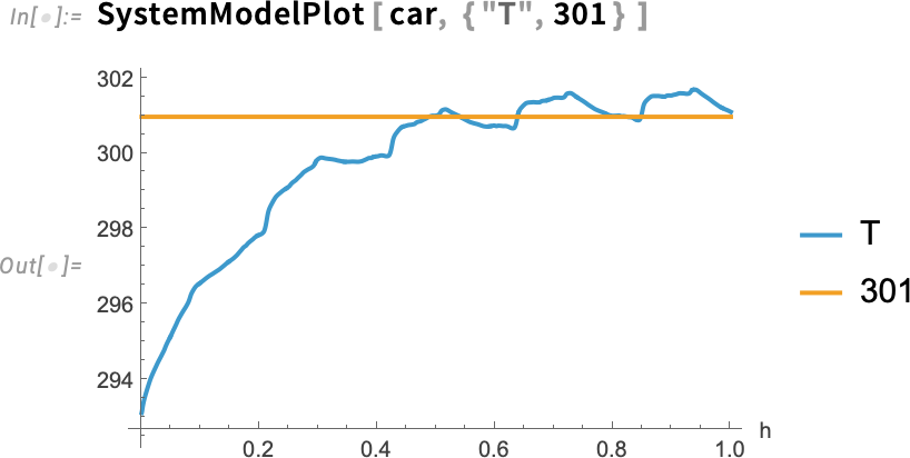
Simulating the underlying model we can see the failure:

There’s a lot of technology involved here. And it’s all set up to be fully industrial scale, so you can use it on any kind of real-world system for which you have a system model.

Smoothing Our Control System Workflows

It’s a capability we’ve been steadily building for the past 15 years: being able to design and analyze control systems. It’s a complicated area, with many different ways to look at any given control system, and many different kinds of things one wants to do with it. Control system design is also typically a highly iterative process, in which you repeatedly refine a design until all design constraints are satisfied.

In Version 14.3 we’ve made this much easier to do, providing easy access to highly automated tools and to multiple views of your system.

Here’s an example of a model for a system (a “plant model” in the language of control systems), given in nonlinear state space form:

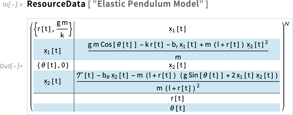
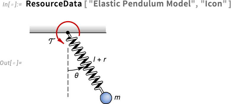
This happens to be a model of an elastic pendulum:

In Version 14.3 you can now click the representation of the model in your notebook, and get a “ribbon” which allows you for example to change the displayed form of the model:

If you’ve filled in numerical values for all the parameters in the model

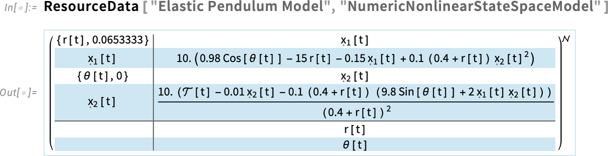
then you can also immediately do things like get simulation results:

Click the result and you can copy the code to get the result directly:

There are lots of properties we can extract from the original state space model. Like here are the differential equations for the system, suitable for input to NDSolve:

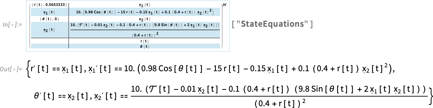
As a more industrial example, let’s consider a linearized model for the pitch dynamics of a particular kind of helicopter:

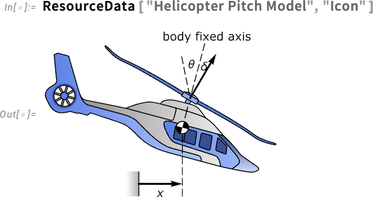
This is the form of the state space model in this case (and it’s linearized around an operating point, so this just gives arrays of coefficients for linear differential equations):

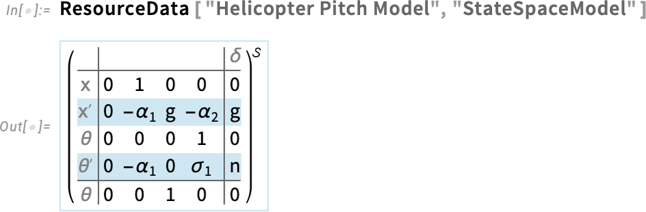
Here’s the model with explicit numerical values filled in:

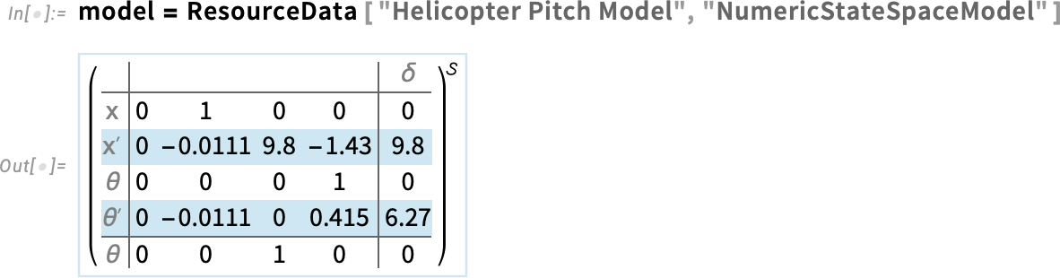
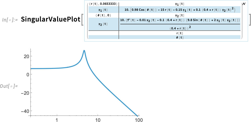
But how does this model behave? To get a quick impression, you can use the new function PoleZeroPlot in Version 14.3, which displays the positions of poles (eigenvalues) and zeros in the complex plane:

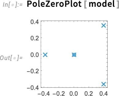
If you know about control systems, you’ll immediately notice the poles in the right half-plane—which will tell you that the system as currently set up is unstable.

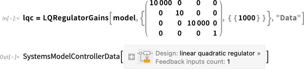
How can we stabilize it? That’s the typical goal of control system design. As an example here, let’s find an LQ controller for this system—with objectives specified by the “weight matrices” we give here:

Now we can plot (in orange) the poles for the system with this controller in the loop—together with (in blue) the poles for the original uncontrolled system:

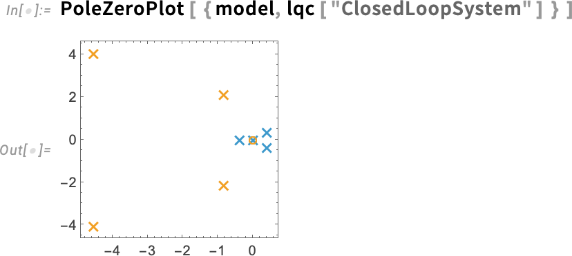
And we see that, yes, the controller we computed does indeed make our system stable.

So what does the system actually do? We can ask for its response given certain initial conditions (here that the helicopter is slightly tipped up):

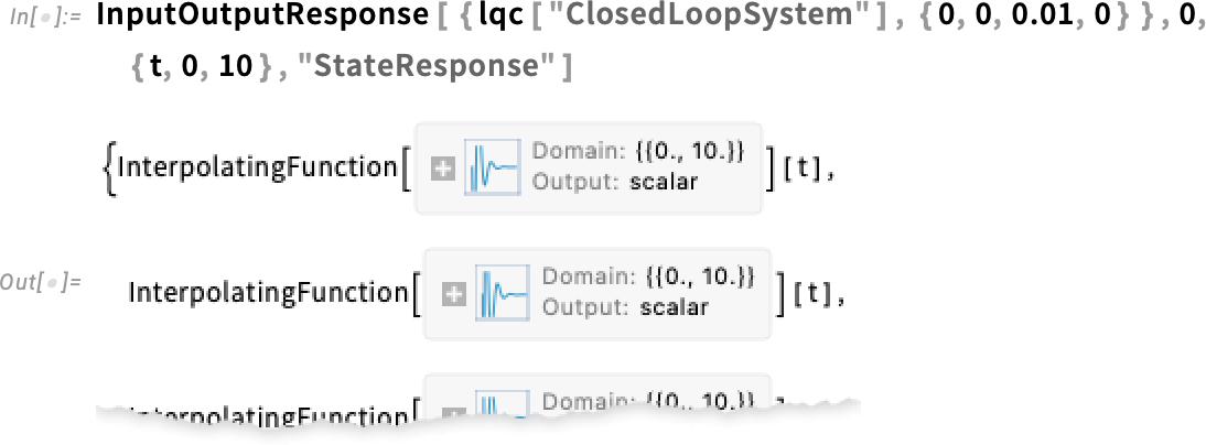
Plotting this we see that, yes, the helicopter wiggles a bit, then settles down:

Going Hyperbolic in Graph Layout

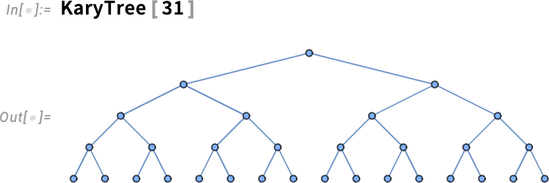
How should you lay out a tree? In fairly small cases it’s feasible to have it look like a (botanical) tree, albeit with its root at the top:

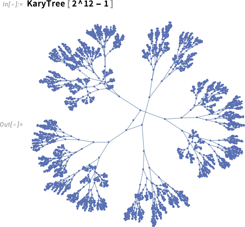
For larger cases, it’s not so clear what to do. Our default is just to fall through to general graph layout techniques:

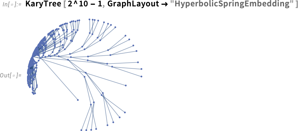
But in Version 14.3 there’s something more elegant we can do: effectively lay the graph out in hyperbolic space:

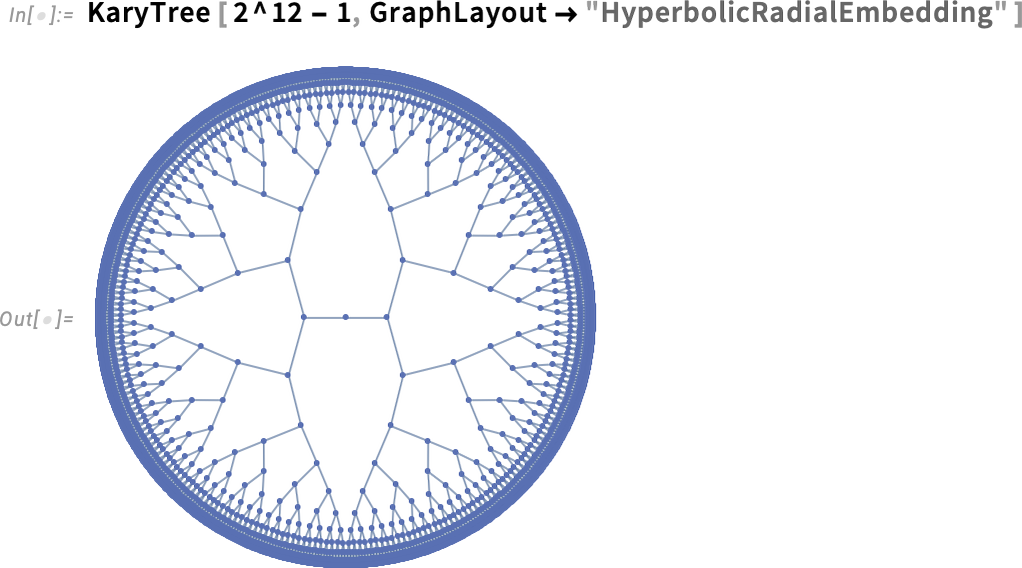
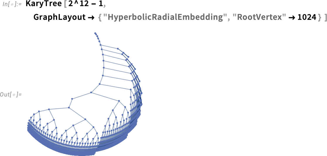
In "HyperbolicRadialEmbedding" we’re in effect having every branch of the tree go out radially in hyperbolic space. But in general we might just want to operate in hyperbolic space, while treating graph edges like springs. Here’s an example of what happens in this case:

At a mathematical level, hyperbolic space is infinite. But in doing our layouts, we’re projecting it into a “Poincaré disk” coordinate system. In general, one needs to pick the origin of that coordinate system, or in effect the “root vertex” for the graph, that will be rendered at the center of the Poincaré disk:

The Latest in Calculus: Hilbert Transforms, Lommel Functions

We’ve done Laplace. Fourier. Mellin. Hankel. Radon. All these are integral transforms. And now in Version 14.3 we’re on to the very last (and most difficult) of the common types of integral transforms: Hilbert transforms. Hilbert transforms show up a lot when one’s dealing with signals and things like them. Because with the right setup, a Hilbert transform basically takes the real part of a signal, say as a function of frequency, and—assuming one’s dealing with a well-behaved analytic function—gives one its imaginary part.

A classic example (in optics, scattering theory, etc.) is:

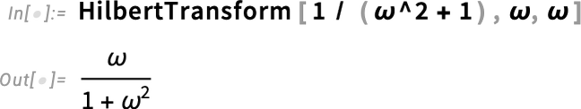
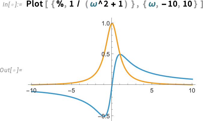
Needless to say, our HilbertTransform can do essentially any Hilbert transform that can be done symbolically:

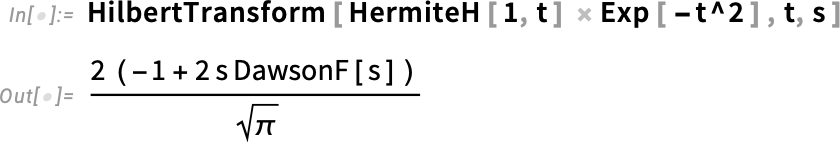
And, yes, this produces a somewhat exotic special function, that we added in Version 7.0.

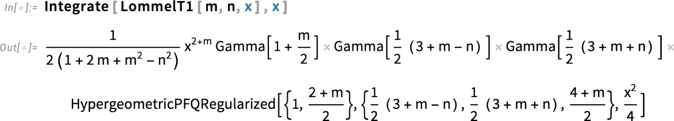
And talking of special functions, like many versions, Version 14.3 adds yet more special functions. And, yes, after nearly four decades we’re definitely running out of special functions to add, at least in the univariate case. But in Version 14.3 we’ve got just one more set: Lommel functions. The Lommel functions are solutions to the inhomogeneous Bessel differential equation:

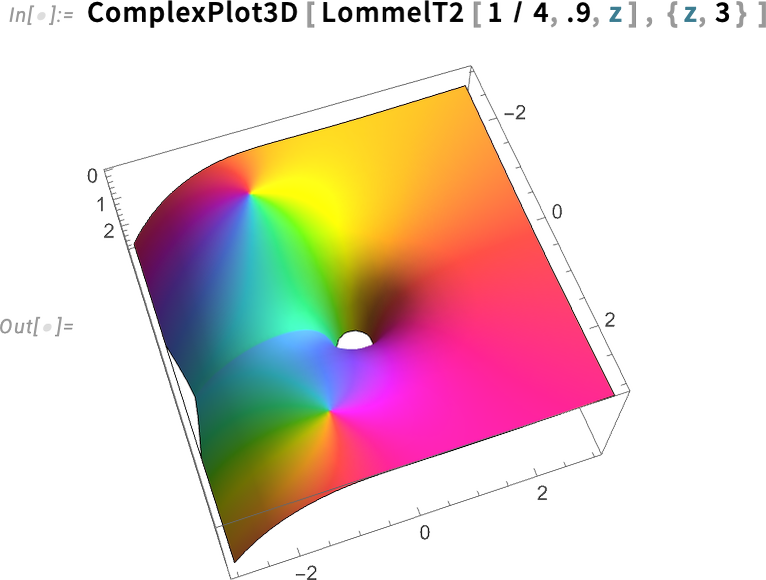
They come in four varieties—LommelS1, LommelS2, LommelT1 and LommelT2:

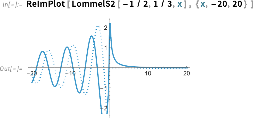
And, yes, we can evaluate them (to any precision) anywhere in the complex plane:

There are all sorts of relations between Lommel functions and other special functions:

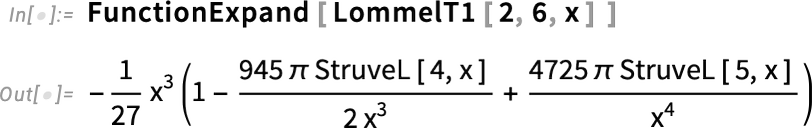
And, yes, like with all our other special functions, we’ve made sure that Lommel functions work throughout the system:

Filling in More in the World of Matrices

Matrices show up everywhere. And starting with Version 1.0 we’ve had all sorts of capabilities for powerfully dealing with them—both numerically and symbolically. But—a bit like with special functions—there are always more corners to explore. And starting with Version 14.3 we’re making a push to extend and streamline everything we do with matrices.

Here’s a rather straightforward thing. Already in Version 1.0 we had NullSpace. And now in Version 14.3 we’re adding RangeSpace to provide a complementary representation of subspaces. So, for example, here’s the 1-dimensional null space for a matrix:

And here is the corresponding 2 (= 3 – 1)-dimensional range space for the same matrix:

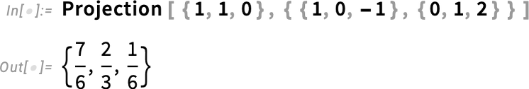
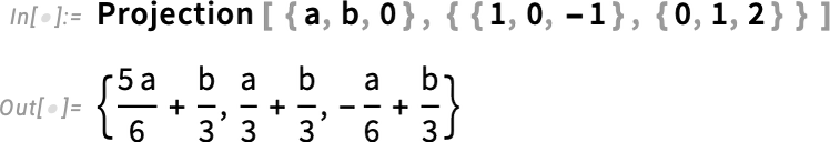
What if you want to project a vector onto this subspace? In Version 14.3 we’ve extended Projection to allow you to project not just onto a vector but onto a subspace:

All these functions work not only numerically but also (using different methods) symbolically:

A meatier set of new capabilities concern decompositions for matrices. The basic concept of a matrix decomposition is to pick out the core operation that’s needed for a certain class of applications of matrices. We had a number of matrix decompositions even in Version 1.0, and over the years we’ve added several more. And now in Version 14.3, we’re adding four new matrix decompositions.

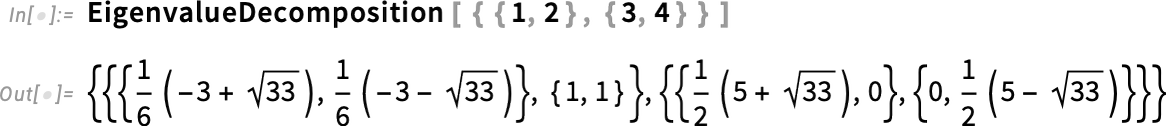
The first is EigenvalueDecomposition, which is essentially a repackaging of matrix eigenvalues and eigenvectors set up to define a similarity transform that diagonalizes the matrix:

The next new matrix decomposition in Version 14.3 is FrobeniusDecomposition:

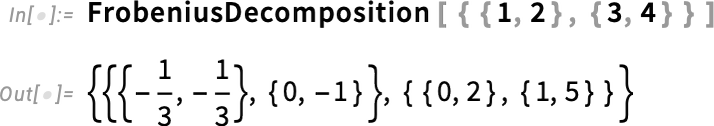
Frobenius decomposition is essentially achieving the same objective as eigenvalue decomposition, but in a more robust way that, for example, doesn’t get derailed by degeneracies, and avoids generating complicated algebraic numbers from integer matrices.

In Version 14.3 we’re also adding a couple of simple matrix generators convenient for use with functions like FrobeniusDecomposition:

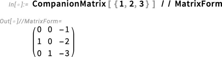
Another set of new functions in effect mix matrices and (univariate) polynomials. For a long time we’ve had:

Now we’re adding MatrixMinimalPolynomial:

We’re also adding MatrixPolynomialValue—which is a kind of polynomial special case of MatrixFunction—and which computes the (matrix) value of a polynomial when the variable (say m) takes on a matrix value:

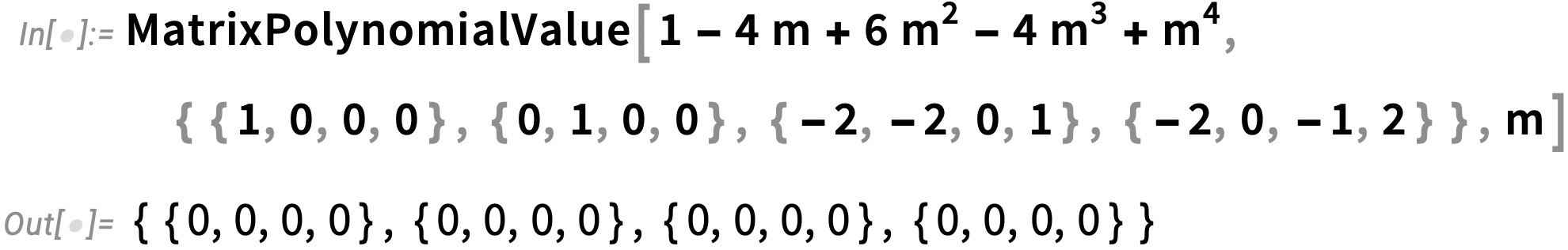
And, yes, this shows that—as the Cayley–Hamilton theorem says—our matrix satisfies its own characteristic equation.

In Version 6.0 we introduced HermiteDecomposition for integer matrices. Now in Version 14.3 we’re adding a version for polynomial matrices—that uses PolynomialGCD instead of GCD in its elimination process:

Sometimes, though, you don’t want to compute full decompositions; you only want the reduced form. So in Version 14.3 we’re adding the separate reduction functions HermiteReduce and PolynomialHermiteReduce (as well as SmithReduce):

One more thing that’s new with matrices in Version 14.3 is some additional notation—particularly convenient for writing out symbolic matrix expressions. An example is the new StandardForm version of Norm:

We had used this in TraditionalForm before; now it’s in StandardForm as well. And you can enter it by filling in the template you get by typing ESCnormESC. Some of the other notations we’ve added are:

With[ ] Goes Multi-argument

In every version—for the past 37 years—we’ve been continuing to tune up details of Wolfram Language design (all the while maintaining compatibility). Version 14.3 is no exception.

Here’s something that I’ve wanted for many, many years—but it’s been technically difficult to implement, and only now become possible: multi-argument With.

I often find myself nesting With constructs:

But why can’t one just flatten this out into a single multi-argument With? Well, in Version 14.3 one now can:

Like the nested With, this first replaces x by 1, then replaces y by x+1. If both replacements are done “in parallel”, y gets the original, symbolic x, not the replaced one:

How could one have told the difference? Look carefully at the syntax coloring. In the multi-argument case, the x in y = x + 1 is green, indicating that it’s a scoped variable; in the non-multi-argument case, it’s blue, indicating that it’s a global variable.

As it turns out, syntax coloring is one of the tricky issues in implementing multi-argument With. And you’ll notice that as you add arguments, variables will appropriately turn green to indicate that they’re scoped. In addition, if there are conflicts between variables, they’ll turn red:

Cyclic[ ] and Cyclic Lists

What’s the 5th element of a 3-element list? One might just say it’s an error. But an alternative is to treat the list as cyclic. And that’s what the new Cyclic function in Version 14.3 does:

You can think of Cyclic[{a,b,c}] as representing an infinite sequence of repetitions of {a,b,c}. This just gives the first part of {a,b,c}:

But this “wraps around”, and gives the last part of {a,b,c}:

You can pick out any “cyclic element”; you’re always just picking out the element mod the length of the block of elements you specify:

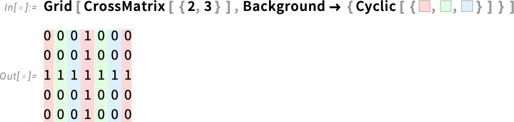
Cyclic provides a way to do computations with effectively infinite repeating lists. But it’s also useful in less “computational” settings, like in specifying cyclic styling, say in Grid:

New in Tabular

Version 14.2 introduced game-changing capabilities for handling gigabyte-sized tabular data, centered around the new function Tabular. Now in Version 14.3 we’re rounding out the capabilities of Tabular in several areas.

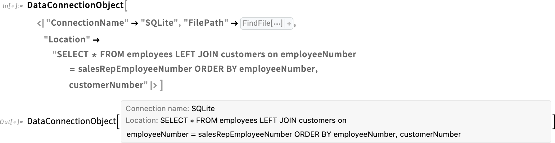
The first has to do with where you can import data for Tabular from. In addition to local files and URLs, Version 14.2 supported Amazon S3, Azure blob storage, Dropbox and IPFS. In Version 14.3 we’re adding OneDrive and Kaggle. We’re also adding the capability to “gulp in” data from relational databases. Already in Version 14.2 we allowed the very powerful possibility of handling data “out of core” in relational databases through Tabular. Now in Version 14.3 we’re adding the capability to directly import for in-core processing the results of queries from such relational databases as SQLite, Postgres, MySQL, SQL Server and Oracle. All this works through DataConnectionObject, which provides a symbolic representation of an active data connection, and which handles such issues as authentication.

Here’s an example of a data connection object that represents the results of a particular query on a sample database:

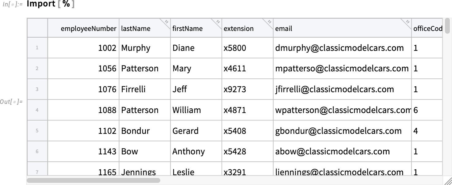
Import can take this and resolve it to an (in-core) Tabular:

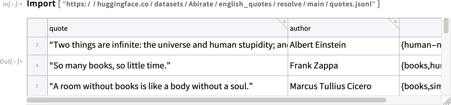
One frequent source of large amounts of tabular data is log files. And in Version 14.3 we’re adding highly efficient importing of Apache log files to Tabular objects. We’re also adding new import capabilities for Common Log and Extended Log files, as well as import (and export) for JSON Lines files:

In addition, we’re adding the capabilities to import as Tabular objects for several other formats (MDB, DBF, NDK, TLE, MTP, GPX, BDF, EDF). Another new feature in Version 14.3 (used for example for GPX data) is a “GeoPosition” column type.

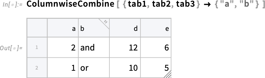
As well as providing new ways to get data into Tabular, Version 14.3 expands our capabilities for manipulating tabular data, and in particular for combining data from multiple Tabular objects. One new function that does this is ColumnwiseCombine. The basic idea of ColumnwiseCombine is to take multiple Tabular objects and to look at all possible combinations of rows in these objects, then to create a single new Tabular object that contains those combined rows that satisfy some specified condition.

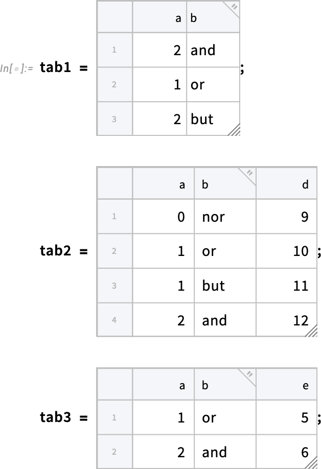
Consider these three Tabular objects:

Here’s an example of ColumnwiseCombine in which the criterion for including a combined row is that the values in columns "a" and "b" agree between the different instances of the row that are being combined:

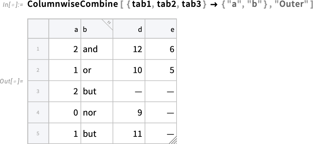
There are lots of subtle issues that can come up. Here we’re doing an “outer” combination, in which we’re effectively assuming that an element that’s missing from a row matches our criterion (and we’re then including rows with those explicit “missing elements” added):

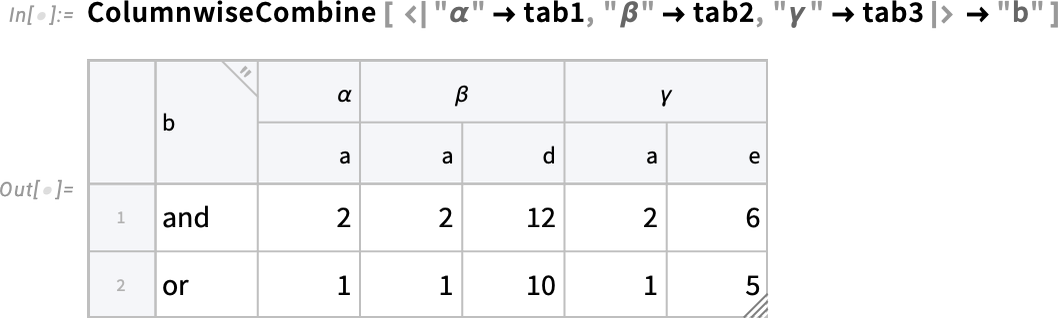
Here’s another subtlety. If in different Tabular objects there are columns that have the same name, how does one distinguish elements from those different Tabular objects? Here we’re effectively giving each Tabular a name, which is then used to form an extended key in the resulting combined Tabular:

ColumnwiseCombine is in effect an n-ary generalization of JoinAcross (which in effect implements the “join” operation of relational algebra). And in Version 14.3 we also upgraded JoinAcross to handle more features of Tabular, for example being able to specify extended keys. And in both ColumnwiseCombine and JoinAcross we’ve set things up so that you can use an arbitrary function to determine whether rows should be combined.

Why would one want to use functions like ColumnwiseCombine and JoinAcross? A typical reason is that one has different Tabular objects that give intersecting sets of data that one wants to knit together for easier processing. So, for example, let’s say we have one Tabular that contains properties of isotopes, and another that contains properties of elements—and now we want to make a combined table of the isotopes, but now including extra columns brought in from the table of elements:

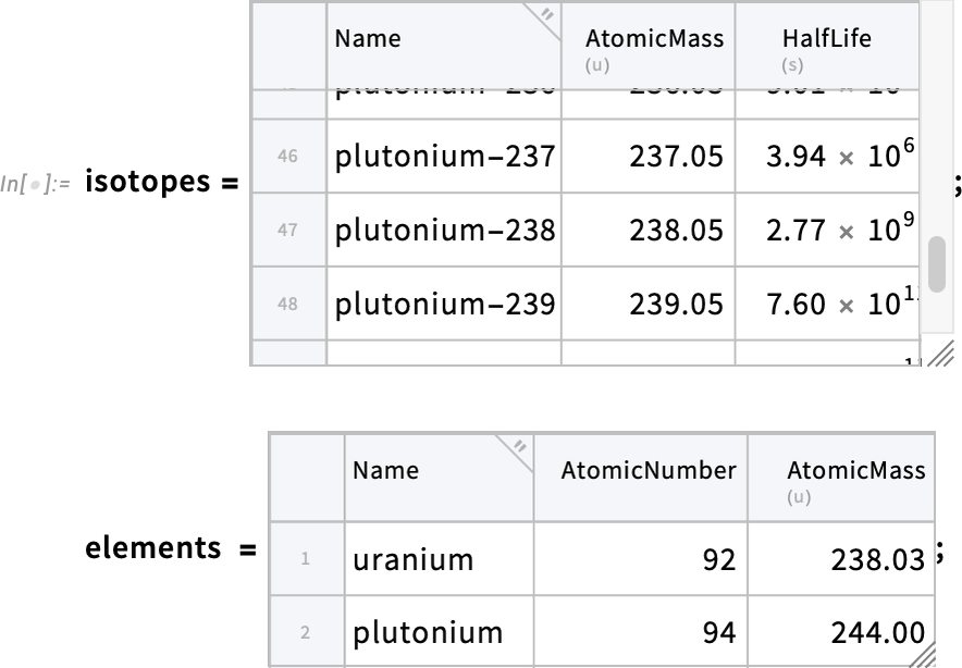
We can make the combined Tabular using JoinAcross. But in this particular case, as is often true with real-world data, the way we have to knit these tables of data together is a bit messy. The way we’ll do it is to use the third (“comparison function”) argument of JoinAcross, telling it to combine rows when the string corresponding to the entry for the "Name" column in the isotopes table has the same beginning as the string corresponding to the "Name" column in the elements table:

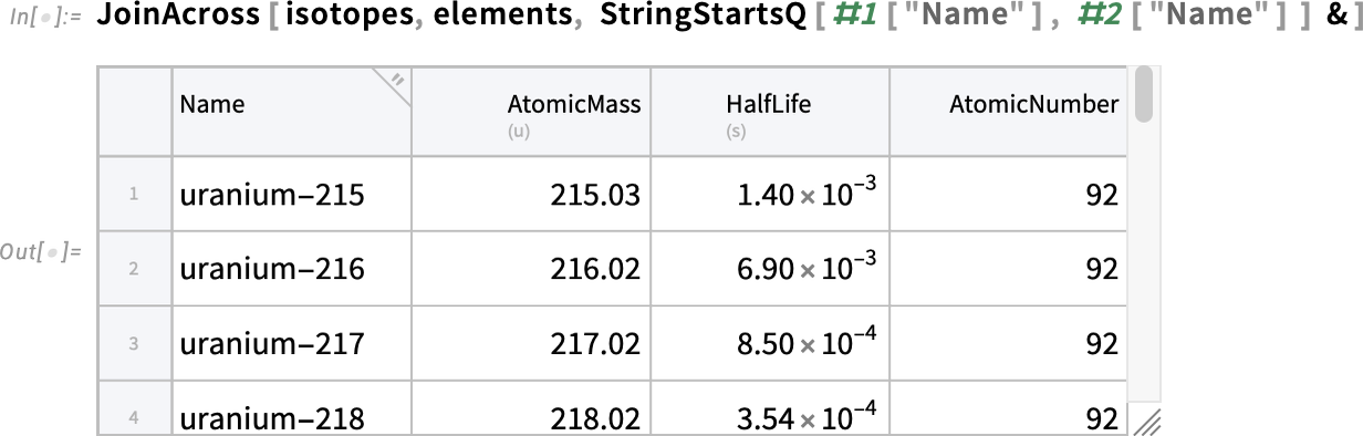
By default, we only get one column in the result with any given name. So, here, the "Name" column comes from the first Tabular in the JoinAcross (i.e. isotopes); the "AtomicNumber" column, for example, comes from the second (i.e. elements) Tabular. We can “disambiguate” the columns by their “source” by specifying a key in the JoinAcross:

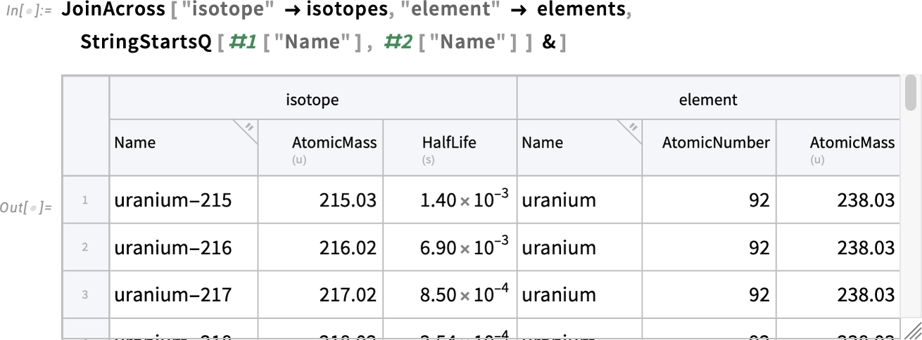
So now we have a combined Tabular that has “knitted together” the data from both our original Tabular objects—a typical application of JoinAcross.

Tabular Styling

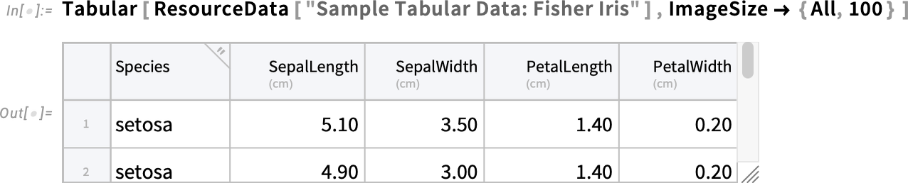
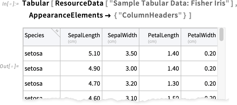
There’s a lot of powerful processing that can be done with Tabular. But Tabular is also a way to store—and present—data. And in Version 14.3 we’ve begun the process of providing capabilities to format Tabular objects and the data they contain. There are simple things. Like you can now use ImageSize to programmatically control the initial displayed size of a Tabular (you can always change the size interactively using the resize handle in the bottom right-hand corner):

You can also use AppearanceElements to control what visual elements get included. Like here we’re asking for column headers, but no row labels or resize handle:

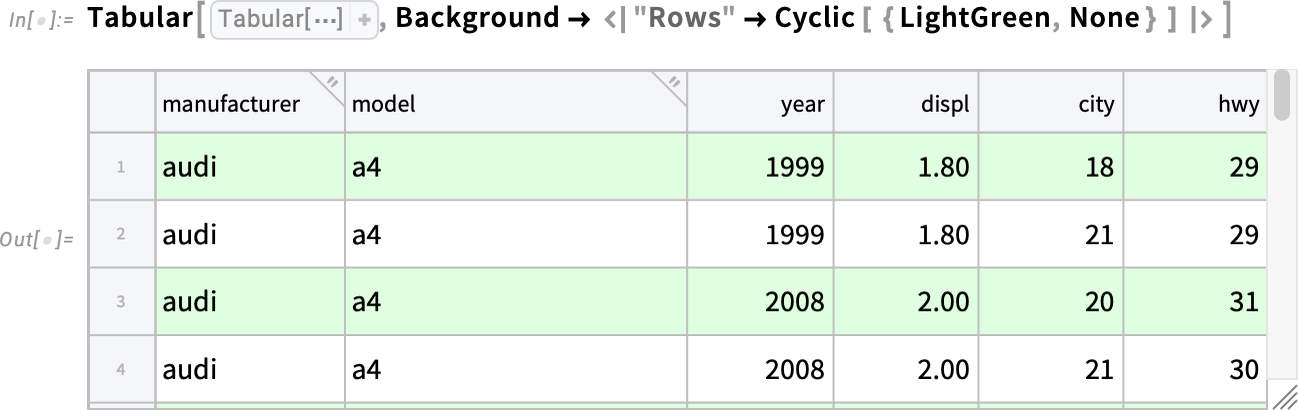
OK, but what about formatting for the data area? In Version 14.3 you can for example specify the background using the Background option. Here we’re asking for rows to alternately have no background or use light green (just like ancient line printer paper!):

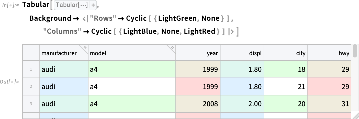
This puts a background on both rows and columns, with appropriate color mixing where they overlap:

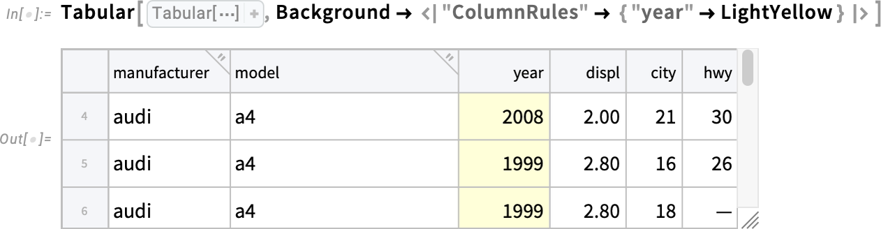
This highlights just a single column by giving it a background color, specifying the column by name:

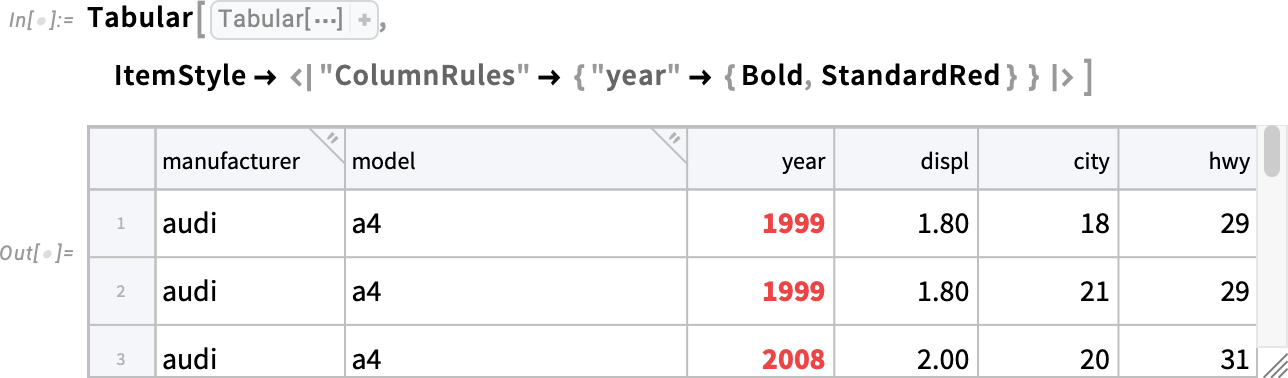
In addition to Background, Version 14.3 also supports specifying ItemStyle for the contents of Tabular. Here we’re saying to make the "year" column bold and red:

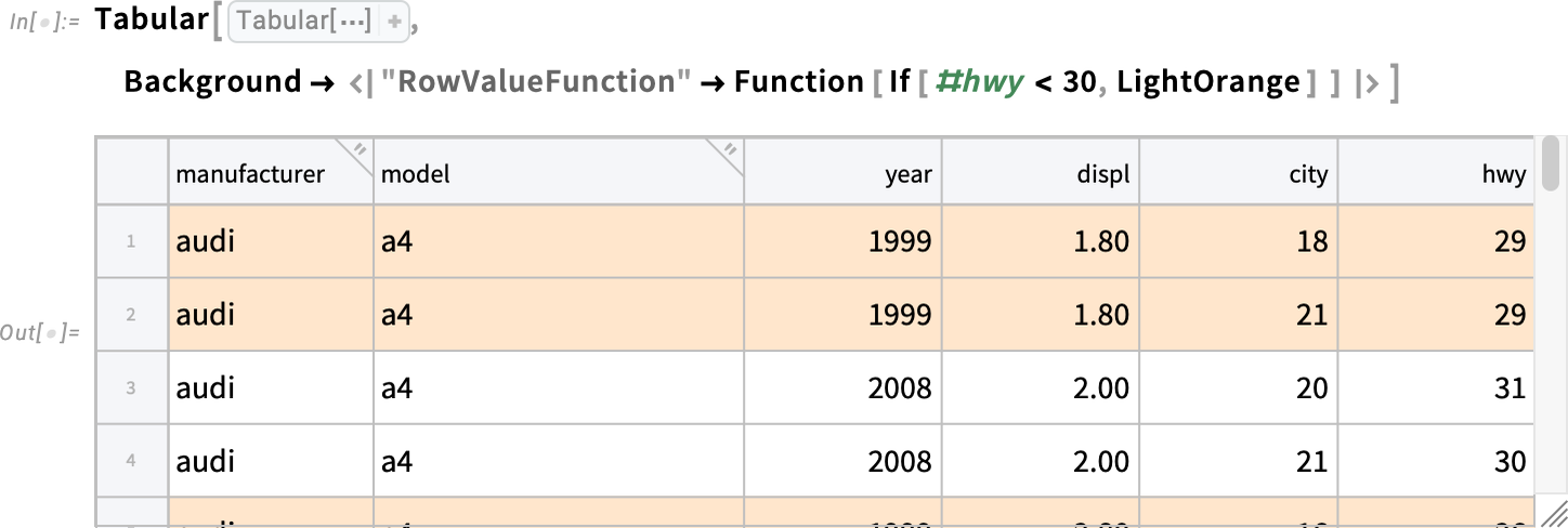
But what if you want the styling of elements in a Tabular to be determined not by their position, but by their value? Version 14.3 provides keys for that. For example, this puts a background color on every row for which the value of "hwy" is below 30:

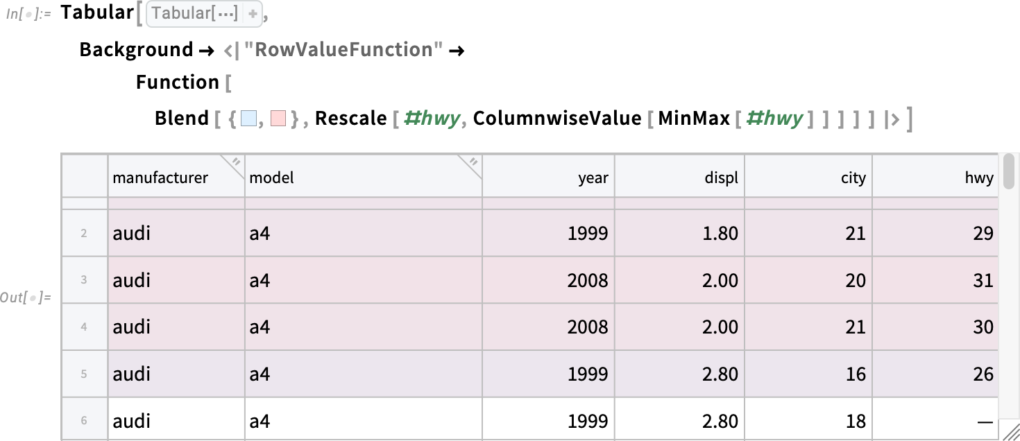
We could do the same kind of thing, but having the color actually be computed from the value of "hwy" (or rather, from its value rescaled based on its overall “columnwise” min and max):

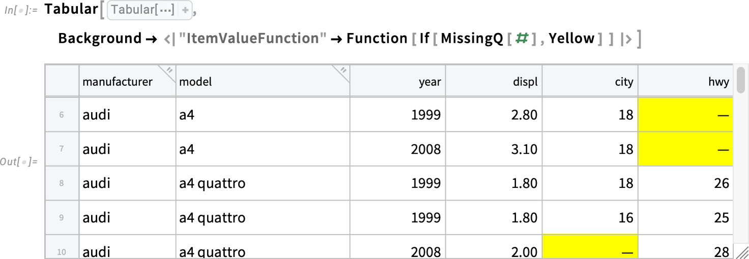
The last row shown here has no color—because the value in its "hwy" column is missing. And if you wanted, for example, to highlight all missing values you can just do this:

Semantic Ranking, Textual Feature Extraction and All That

Which of those choices do you mean? Let’s say you’ve got a list of choices—for example a restaurant menu. And you give a textual description of what you want from those choices. The new function SemanticRanking will rank the choices according to what you say you want:

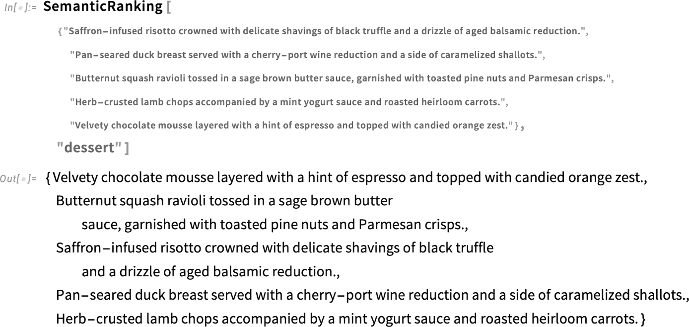
And because this is using modern language model methods, the choices could, for example, be given not only in English but in any language.

If you want, you can ask SemanticRanking to also give you things like relevance scores:

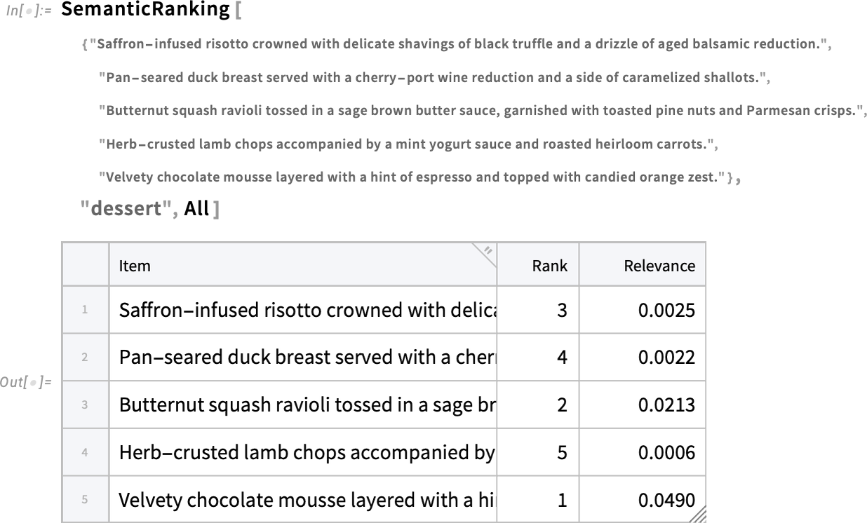
How does SemanticRanking relate to the SemanticSearch functionality that we introduced in Version 14.1? SemanticSearch actually by default uses SemanticRanking as a final ranking for the results it gives. But SemanticSearch is—as its name suggests—searching a potentially large amount of material, and returning the most relevant items from it. SemanticRanking, on the other hand, is taking a small “menu” of possibilities, and giving you a ranking of all of them based on relevance to what you specify.

SemanticRanking in effect exposes one of the elements of the SemanticSearch pipeline. In Version 14.3 we’re also exposing another element: an enhanced version of FeatureExtract for text, that is pre-trained, and does not require its own explicit examples:

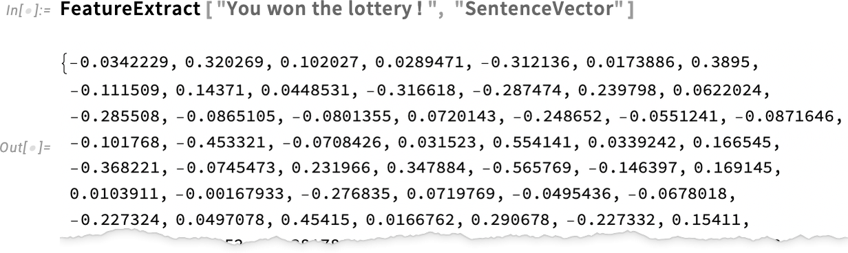
Our new feature extractor for text also improves Classify, Predict, FeatureSpacePlot, etc. in the case of sentences or other pieces of text.

Compiled Functions That Can Pause and Resume

The typical flow of computation in the Wolfram Language is a sequence of function calls, with each function running and returning its result before another function is run. But Version 14.3 introduces—in the context of the Wolfram Language compiler—the possibility for a different kind of flow in which functions can be paused at any point, then resumed later. In effect what we’ve done is to implement a form of coroutines, that allows us to do incremental computation, and for example to support “generators” that can yield a sequence of results, always maintaining the state needed to produce more.

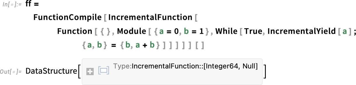
The basic idea is to set up an IncrementalFunction object that can be compiled. The IncrementalFunction object uses IncrementalYield to return “incremental” results—and can contain IncrementalReceive functions that allow it to receive more input while it is running.

Here’s a very simple example, set up to create an incremental function (represented as a DataStructure of type “IncrementalFunction”) that will keep successively generating powers of 2:

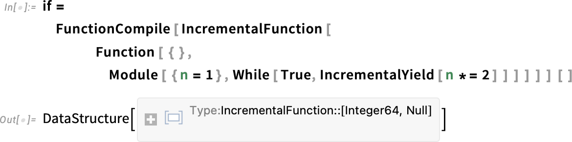
Now every time we ask for the "Next" element of this, the code in our incremental function runs until it reaches the IncrementalYield, at which point it yields the result specified:

In effect the compiled incremental function if is always internally “maintaining state” so that when we ask for the "Next" element it can just continue running from the state where it left off.

Here’s a slightly more complicated example: an incremental version of the Fibonacci recurrence:

Every time we ask for the "Next" element, we get the next result in the Fibonacci sequence:

The incremental function is set up to yield the value of a when you ask for the "Next" element, but internally it maintains the values of both a and b so that it is ready to “keep running” when you ask for another "Next" element.

In general, IncrementalFunction provides a new and often convenient way to organize code. You get to repeatedly run a piece of code and get results from it, but with the compiler automatically maintaining state, so you don’t explicitly have to take care of that, or include code to do it.

One common use case is in enumeration. Let’s say you have an algorithm for enumerating certain kinds of objects. The algorithm builds up an internal state that lets it keep generating new objects. With IncrementalFunction you can run the algorithm until it generates an object, then stop the algorithm, but automatically maintain the state to resume it again.

For example, here’s an incremental function for generating all possible pairs of elements from a specified list:

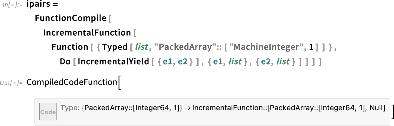
Let’s tell it to generate the pairs from a list of a million elements:

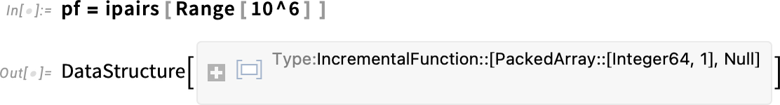
The complete collection of all these pairs wouldn’t fit in computer memory. But with our incremental function we can just successively request individual pairs, maintaining “where we’ve got to” inside the compiled incremental function:

Another thing one can do with IncrementalFunction is, for example, to incrementally consume some external stream of data, for example from a file or API.

IncrementalFunction is a new, core capability for the Wolfram Language that we’ll be using in future versions to build a whole array of new “incremental” functionality that lets one conveniently work (“incrementally”) with collections of objects that couldn’t be handled if one had to generate them all at once.

Faster, Smoother Encapsulated External Computation

We’ve worked very hard (for decades!) to make things work as smoothly as possible when you’re working within the Wolfram Language. But what if you want to call external code? Well, it’s a jungle out there, with all kinds of issues of compatibility, dependencies, etc. But for years we’ve been steadily working to provide the best interface we can within Wolfram Language to external code. And in fact what we’ve managed to provide is now often a much smoother experience than with the native tools normally used with that external code.

Version 14.3 includes several advances in dealing with external code. First, for Python, we’ve dramatically sped up the provisioning of Python runtimes. Even the first time you use Python ever, it now takes just a few seconds to provision itself. In Version 14.2 we introduced a very streamlined way to specify dependencies. And now in Version 14.3 we’ve made provisioning of runtimes with particular dependencies very fast:

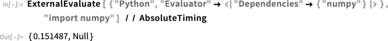
And, yes, a Python runtime with those dependencies will now be set up on your machine, so if you call it again, it can just run immediately, without any further provisioning.

A second major advance in Version 14.3 is the addition of a highly streamlined way of using R within Wolfram Language. Just specify R as the external language, and it’ll automatically be provisioned on your system, and then run a computation (yes, having "rnorm" as the name of the function that generates Gaussian random numbers offends my language design sensibilities, but…):

You can also use R directly in a notebook (type > to create an External Language cell):

One of the technical challenges is to set things up so that you can run R code with different dependencies within a single Wolfram Language session. We couldn’t do that before (and in some sense R is fundamentally not built to do it). But now in Version 14.3 we’ve set things up so that, in effect, there can be multiple R sessions running within your Wolfram Language session, each with their own dependencies, and own provisioning. (It’s really complicated to make this all work, and, yes, there might be some pathological cases where the world of R is just too tangled for it to be possible. But such cases should at least be very rare.)

Another thing we’ve added for R in Version 14.3 is support for ExternalFunction, so you can have code in R that you can set up to use just like any other function in Wolfram Language.

Notebooks into Presentations: the Aspect Ratio Challenge Solved

Notebooks are ordinarily intended to be scrolling documents. But—particularly if you’re making a presentation—you sometimes want them instead in more of a slideshow form (“PowerPoint style”). We’d had various approaches before, but in Version 11.3—seven years ago—we introduced Presenter Tools as a streamlined way to make notebooks to use for presentations.

The principle of it is very convenient. You can either start from scratch, or you can convert an existing notebook. But what you get in the end is a slideshow-like presentation, that you can for example step through with a presentation clicker. Of course, because it’s a notebook, you get all sorts of additional conveniences and features. Like you can have a Manipulate on your “slide”, or cell groups you can open and close. And you can also edit the “slide”, do evaluations, etc. It all works very nicely.

But there’s always been one big issue. You’re fundamentally trying to make what amount to slides—that will be shown full screen, perhaps projected, etc. But what aspect ratio will those slides have? And how does this relate to the content you have? For things like text, one can always reflow to fit into a different aspect ratio. But it’s trickier for graphics and images, because these already have their own aspect ratios. And particularly if these were somewhat exotic (say tall and narrow) one could end up with slides that required scrolling, or otherwise weren’t convenient or didn’t look good.

But now, in Version 14.3 we have a smooth solution for all this—that I know I, for one, am going to find very useful.

Choose File > New > Presenter Notebook… then press Create to create a new, blank presenter notebook:

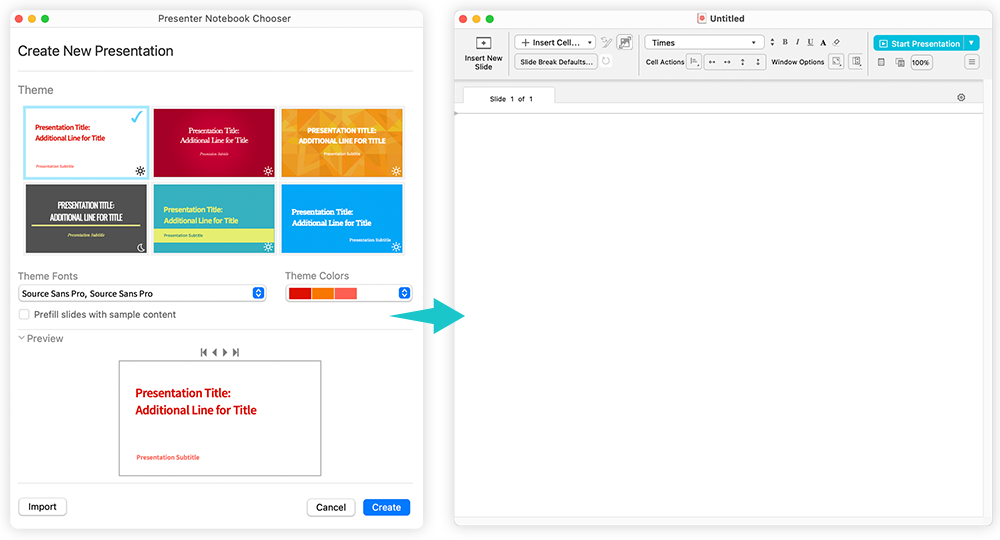
In the toolbar, there’s now a new button that inserts a template for a full-slide image (or graphic):

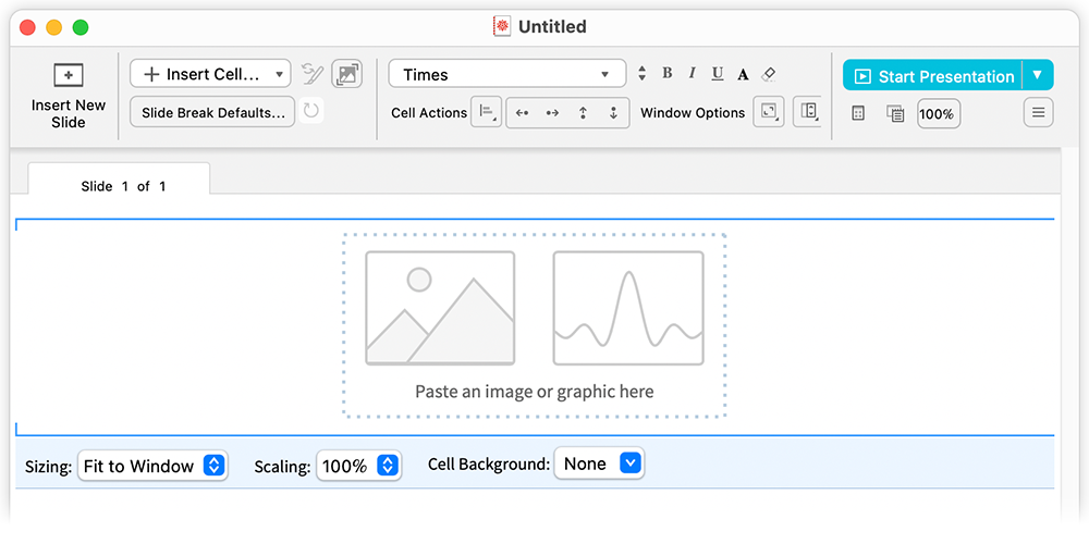
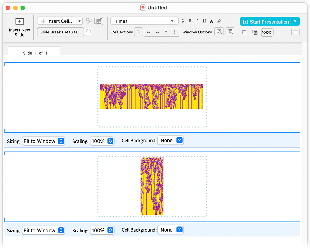
Insert an image—by copy/pasting, dragging (even from an external program) or whatever—with any aspect ratio:

Press and you’ll get a full-screen presentation—with everything sized right, the short-and-wide graphic spanning the width of my display, and the tall-and-narrow graphic spanning the height:

When you insert a full-slide image, there’s always a “control bar” underneath:

The first pulldown

lets you decide whether the make the image fit in the window, or whether instead to make it fill out the window horizontally, perhaps clipping at the top and bottom.

Now remember that this template is for placing full-slide images. If you want there to be room, say for a caption, on the slide, you need to pick a size less than 100%.

By default, the background of the cells you get is determined by the original presenter notebook theme you chose. So in the example here, the default background will be white. And this means that if, for example, you’re projecting your images there’ll always be a “background white rectangle”. But if you want to just see your image projected—at its natural aspect ratio—with nothing visible around it, you can select Cell Background to instead be black.

Yet More User Interface Polishing

It’s been 38 years since we invented notebooks… but in every new version we’re still continuing to polish and enhance how they work. Here’s an example. Nearly 30 years ago we introduced the idea that if you type -> it’ll get replaced by the more elegant . Four years ago (in Version 12.3) we tweaked this idea by having -> not actually be replaced by , but instead just render that one. But here’s a subtle question: if you arrow backwards through the does it show you the characters it’s made from? In previous versions it did, but now in Version 14.3 it doesn’t. It’s something we learned from experience: if you see something that looks like a single character (here ) it’s strange and jarring for it to break apart if you arrow through it. So now it doesn’t. However, if you backspace (rather than arrowing), it will break apart, so you can edit the individual characters. Yes, it’s a subtle story, but getting it just right is one of those many, many things that makes the Wolfram Notebook experience so smooth.

Here’s another important little convenience that we’ve added in Version 14.3: single-character delimiter wrapping. Let’s say you typed this:

Most likely you actually wanted a list. And you can get it by adding { at the beginning, and } at the end. But now there’s a more streamlined thing to do. Just select everything

and now simply type {. The { … } will automatically get wrapped around the selection:

The same thing works with ( … ), [ … ], and “ … ”.

It may seem like a trivial thing. But if you’ve got lots of code on the screen, it’s very convenient to not have to go back and forth adding delimiters—but just be able to select some subexpression, then type a single character.

There’ve been a number of changes to icons, tooltips, etc. just to make things clearer. Something else is that (finally) there’s support for separate British and American English spelling dictionaries. By default, the choice of which one to use is made automatically from the setting for your operating system. But yes, “color” vs. “colour” and “center” vs. “centre” will now follow your preferences and get tagged appropriately. By the way, in case you’re wondering: we’ve been curating our own spelling dictionaries for years. And in fact, I routinely send in words to add, either because I find myself using them, or, yes, because I just invented them (“ruliad”, “emes”, etc.).

Markdown!

You want a file that’s plaintext but “formatted”. These days a common way to achieve that is to use Markdown. It’s a format both humans and AIs can easily read, and it can be “dressed up” to have visual formatting. Well, in Version 14.3 we’re making Markdown an easy-to-access format in Wolfram Notebooks, and in the Wolfram Language in general.

It should be said at the outset that Markdown isn’t even close to being as rich as our standard Notebook format. But many key elements of notebooks can still be captured by Markdown. (By the way, our .nb notebook files are, like Markdown, actually pure plaintext, but since they have to faithfully represent every aspect of notebook content, they’re inevitably not as spare and easy to read as Markdown files.)

OK, so let’s say you have a Notebook:

You can get a Markdown version just by using File > Save As > Markdown:

Here’s what this looks like in a Markdown viewer:

The main features of the notebook are there, but there are details missing (like cell backgrounds, real math typesetting, etc.), and the rendering is definitely not as beautiful as in our system nor as functional (for example, there are no closeable cell groups, no dynamic interactivity, etc.).

OK, so let’s say you have a Markdown file. In Version 14.3 you can now just use File > Open, choose “Markdown Files” as the file type, and open the Markdown file as a Notebook:

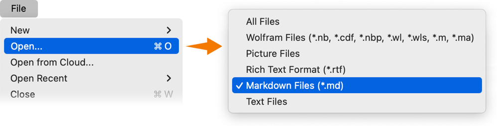
Round-tripping through Markdown loses some of the finer points of a Notebook, but the basic structure is there. And, yes, you can open Markdown files “from the wild” this way too, coming, for example, from notes apps, software documentation, raw LLM output, etc.

In addition to handling Markdown at a “whole file” level, you can also generate (and read) Markdown fragments. So, for example, you can take a table in a Notebook, then just do Copy As > Markdown to get a Markdown version:

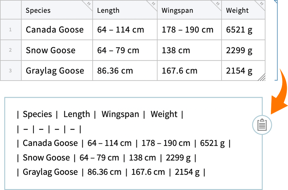
Needless to say, everything you can do interactively with Markdown, you can also do programmatically in the Wolfram Language. So, for example, you can use ExportString to export to Markdown:

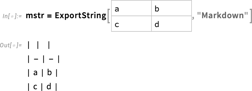
Importing this gives by default plaintext:

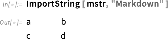
But if you tell it to import as “formatted text”, it’ll package up the data in a tabular form:

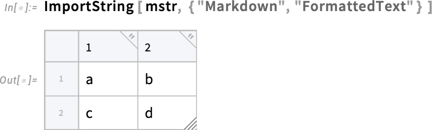
Particularly when you’re communicating with LLMs, it’s often useful to have Markdown tables that are just “summaries” of longer, original tables. Here we’re asking for 3 rows of data:

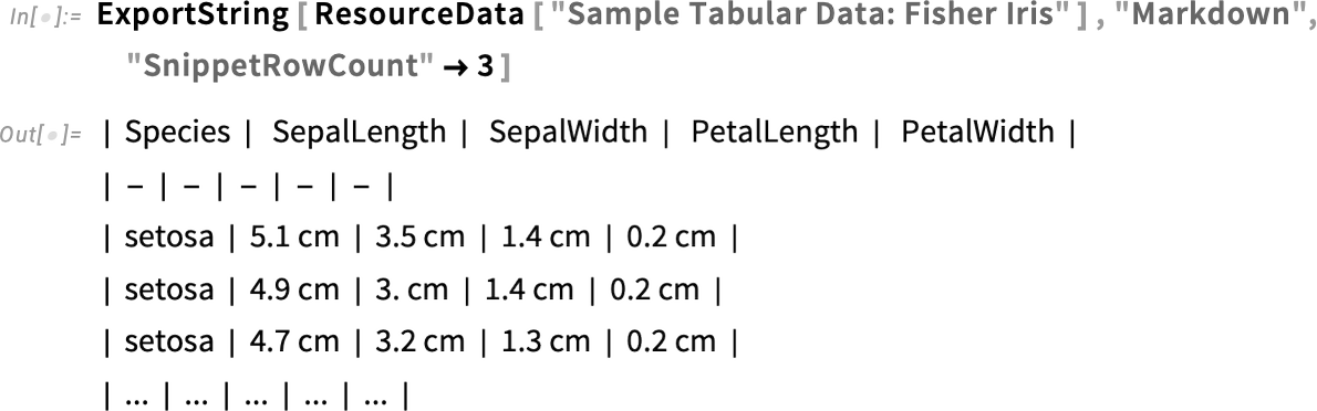
And here we’re asking for 2 rows at the beginning, and 2 at the end:

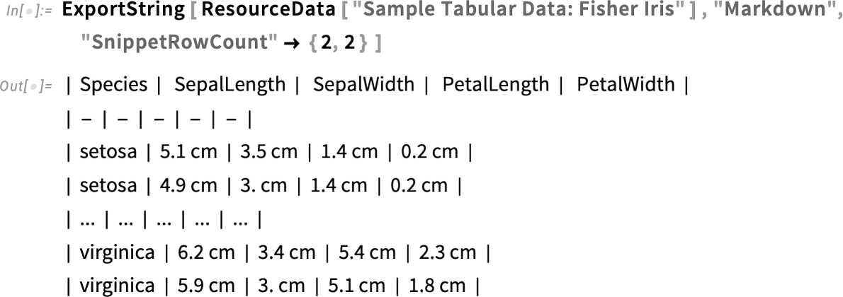
There are lots of subtleties (and clever heuristics) associated with getting Markdown that’s as good—and round-trippable—as possible. If you export an image to Markdown

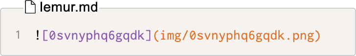
the actual Markdown will simply contain a pointer to a file that’s been created (in the img subdirectory) to store the image. This is particularly convenient if you’re using the Wolfram Cloud, where the images are embedded in the Markdown file as data URLs:

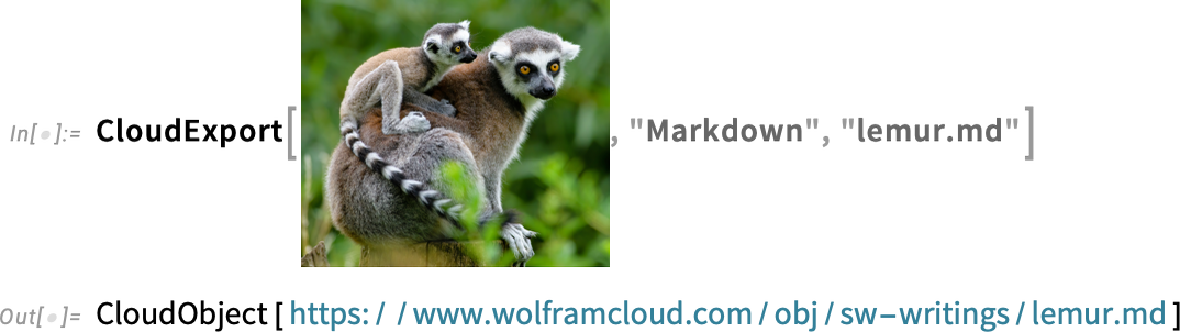
New in Web Documentation: Navigation Sidebar

Ever since Version 13, there’s been a choice: download all 6.5 gigabytes of Wolfram Language documentation and use it locally, or just link to the web for documentation, without downloading anything. (By the way, if you want to download documentation, but haven’t, you can always do it with Install Local Documentation item in the Help menu.)

In Version 14.3 there’s a new feature in web documentation. Assuming you have your browser window set fairly wide, there’s now a navigation sidebar on every function page:

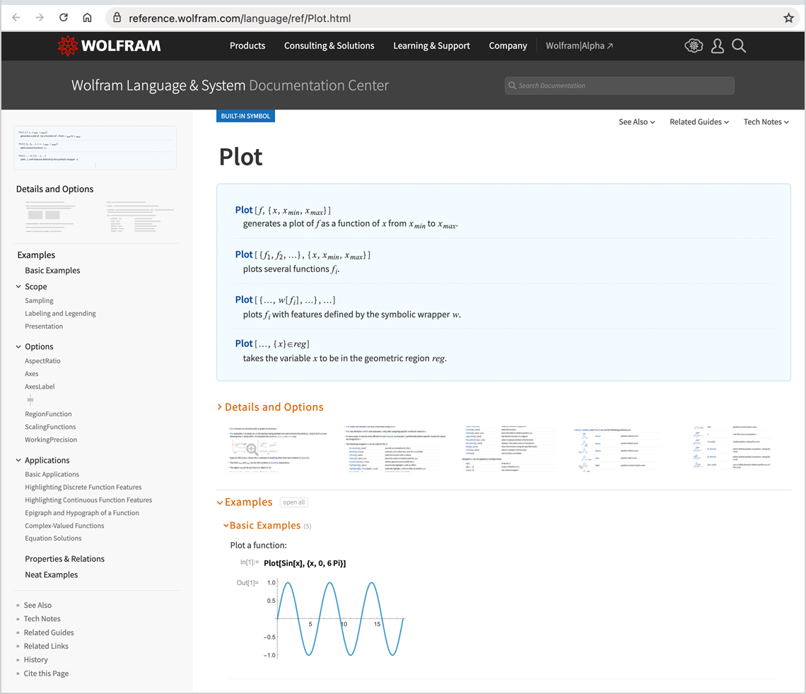
Want to quickly look up how that option works? Just click it in the sidebar, and the page will jump down to where that option is described, opening the relevant cells:

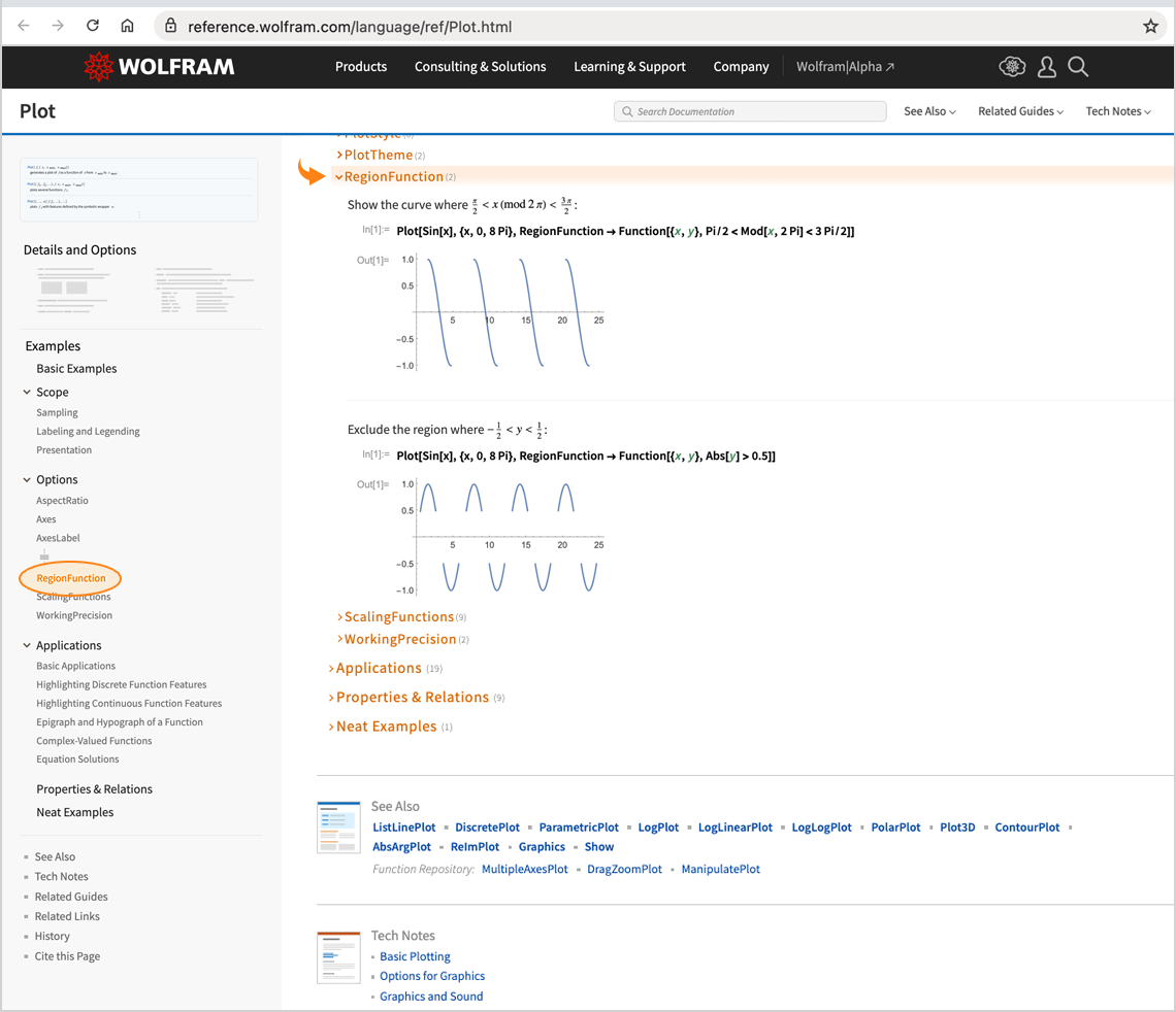
Of course, in nearly 10,000 pages of rather diverse material, lots of complicated UX issues come up. Like with Plot, for example, the full list of options is very long, so by default it’s elided with :

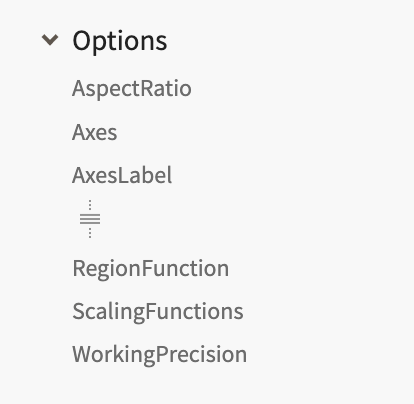
Click the and all the options open up—with something like a cell bracket, that you can click to close it again:

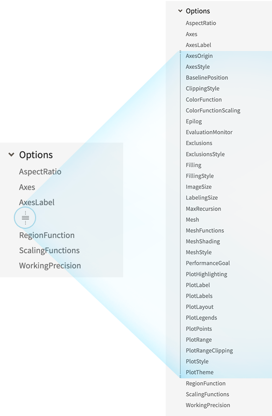
And Even More…

Version 14.3 is a strong release, full of new capabilities. And the things we’ve discussed so far aren’t even everything. There’s even more.

In video, for example, we’ve added VideoStabilize to take out jitter in videos. We’ve also enhanced VideoObjectTracking to let you specify particular points in a video to track. And if you effectively want to track every point, we’ve enhanced ImageDisplacements to work on videos.

In images, we now import .avif (AV1) files.

In speech synthesis, we’re now able to always do everything locally. In Version 14.2 we were using operating-system-based speech synthesis on Mac and Windows. Now we’ve got a collection of local neural net models that run consistently on any operating system—and whenever we can’t use operating-system-based speech synthesis, these are what we use.

Version 14.3 also adds yet more polish to our already very well developed system for handling dates. In particular, we’ve added new day types such as “NonHoliday” and “WeekendHoliday” , and we’ve provided an operator form of DayMatchQ—all in service of making it easy (and, by the way, very efficient) to more finely select specific types of dates, notably now in Tabular.

In a completely different area, Version 14.3 makes RandomTree much more efficient, and also allows trees with a specified list of node labels, here the alphabet:

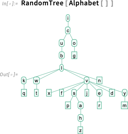
Talking of efficiency, a small but useful enhancement to the world of DataStructure is that “BitVector” data structures now use multithreading, and the function Pick can operate directly on such data structures—including ones that are billions of bits long.

Also, in computation with GPUArray objects, we’ve further improved the performance of core arithmetic operations, as well as adding GPU support for functions like UnitStep and NumericalSort.

In the continuing story of partial differential equations and PDE modeling, Version 14.3 includes a new option for solving axisymmetric fluid flow problems—allowing one for example to compute this solution for flow through a pipe with a constriction:

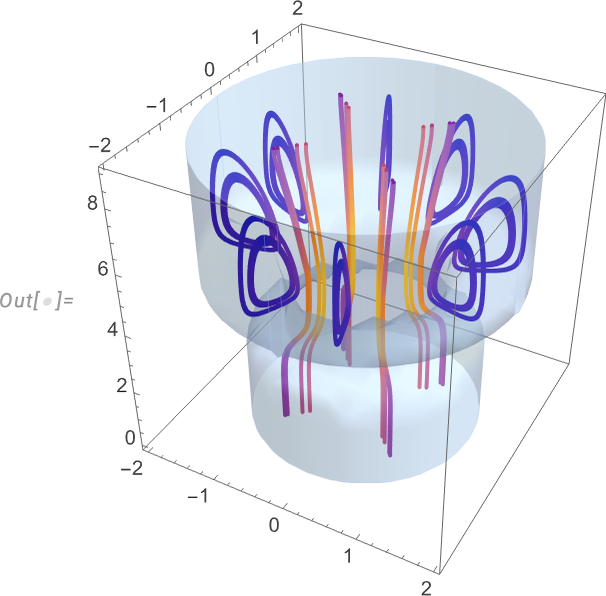
In biochemistry, we’ve added connections to UniProt and the AlphaFold database. And in chemistry we’ve added various utility functions such as ChemicalFormulaQ and PatternReactionQ.

In the compiler we’ve added CurrentCompiledFunctionData to provide introspection on compiled functions, allowing you to determine, for example, what particular type the compiler assigned to the function you’re currently in:

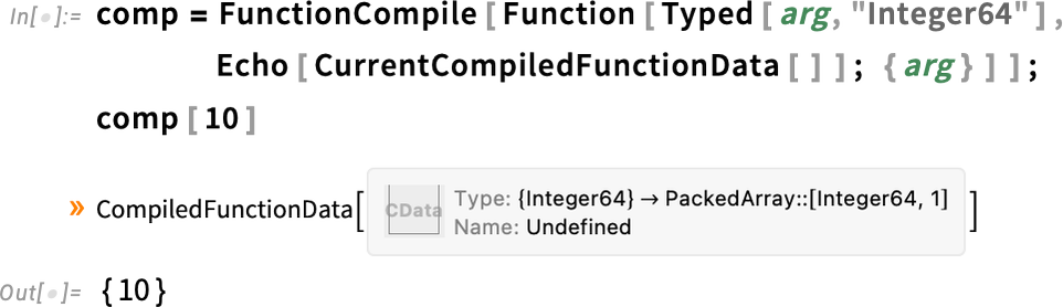
Also in the compiler we’ve extended DownValuesFunction to let you “wrap for compilation” functions whose definitions involve constructs like Alternatives and Except. (This is a further precursor to letting you just directly compile raw downvalue assignments.)

In addition to all this, there are a large number of little tweaks and little pieces of polish that we’ve added in Version 14.3, along with over a thousand bug fixes: all things that make the experience of using Wolfram Language just that much smoother and richer.

Version 14.3 for desktop systems is ready for download now. It’s also now what you automatically get in the Wolfram Cloud. So… start using it today! And experience the fruits of the latest round of our intense research and development efforts…